Difference between revisions of "Projects:QuantitativeSusceptibilityMapping"
| (79 intermediate revisions by 2 users not shown) | |||
| Line 1: | Line 1: | ||
| − | + | = Introduction = | |
| − | |||
| − | |||
| − | |||
| − | |||
| − | |||
| − | |||
| − | |||
| − | |||
| − | |||
| − | |||
| − | |||
| − | |||
| − | |||
| − | |||
| − | = | ||
There is increasing evidence that excessive iron deposition in specific regions | There is increasing evidence that excessive iron deposition in specific regions | ||
| Line 24: | Line 9: | ||
In magnetic resonance imaging (MRI) experiments, differences | In magnetic resonance imaging (MRI) experiments, differences | ||
in magnetic susceptibility cause perturbations in the local magnetic field, which | in magnetic susceptibility cause perturbations in the local magnetic field, which | ||
| − | can be computed from the phase of the MR signal. | + | can be computed from the phase of the MR signal (in a gradient echo sequence, the observed field is proportional to the MR phase). |
| + | |||
| + | = Description = | ||
| + | |||
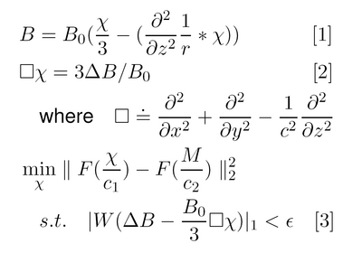
| + | In MRI, magnetic susceptibility differences cause measurable perturbations in the local magnetic field that can be modeled as the convolution of a dipole-like kernel with the spatial susceptibility distribution. In the Fourier domain, the kernel exhibits zeros at the magic angle, preventing direct inversion of the field map; also, limited observations make the problem ill-posed. The observed data is also corrupted by confounding fields (ie. those from tissue/air interfaces, mis-set shims, and other non-local sources). Previous work has shown that MR images can be successfully reconstructed from under-sampled observations by exploiting the sparsity of in-vivo data under various transforms using methods from compressed sensing [2]. In susceptibility estimation, the forward model results in under-sampling of the data in the Fourier domain, but accurate estimates can be obtained using the Laplacian and L1 norm, which promote sparse solutions while removing external field artifacts. Our variational method for susceptibility estimation is described in Figs. 1-2. | ||
| + | |||
| + | {| | ||
| + | |[[File:Namic wiki fig1.png|thumb|400px|Fig 1. Relevant notation]] | ||
| + | |} | ||
| + | |||
| + | {| | ||
| + | |[[File:Latex pdf zoomed to paint equations.PNG|thumb|400px|Fig 2. Applying the Laplacian to the forward model in [1] eliminates non-local phase artifacts to give [2]. The first term in [3] provides regularization, penalizing large differences in spatial frequency relative to Magnitude data, while the second penalizes departures from [2], enforcing agreement of high frequency phase effects.]] | ||
| + | |} | ||
| + | |||
| + | == Forward Model (Eq. 1) == | ||
| + | |||
| + | The forward model relates the perturbing field to the unknown susceptibility through a local term and convolution of the second z-derivative of the Green’s function of the Laplacian with the unknown susceptibility map [3]. | ||
| + | == Bias Field Elimination (Eq. 2) == | ||
| − | + | Applying the Laplacian removes non-local phase effects such as shim fields, which are a solution to the Laplace equation. | |
| − | |||
| − | |||
| − | |||
| − | |||
| − | |||
| − | non-local | ||
| − | |||
| − | |||
| + | == Objective Function (Eq. 3) == | ||
| − | + | The first term provides regularization, penalizing solutions with large differences in spatial frequency structure relative to the magnitude image. | |
| − | + | The second term penalizes departures from Eq. 2, by enforcing agreement of high frequency phase effects while eliminating low order bias fields. | |
| − | |||
| − | |||
| − | |||
| − | |||
| − | |||
| − | |||
| − | |||
| − | |||
| − | |||
| − | |||
| − | |||
| − | |||
| − | |||
| − | |||
| − | |||
| + | == Data Acquisition == | ||
| − | + | Cylindrical and rectangular phantoms were made using Magnevist (gadopentetate dimeglumine) solutions of 0.5, 1.0, 2.0, and 3.0 mM corresponding to susceptibility values of 0.15, 0.31, 0.62, and 0.94 ppm [4,5]. Field maps were obtained using a 3D multi-echo GRE sequence on a 3T Siemens Trio MRI. | |
| − | ( | ||
| − | |||
| − | |||
| − | |||
| − | |||
| − | |||
| − | |||
| − | |||
| − | |||
| − | |||
| − | |||
| − | |||
| − | |||
= Results = | = Results = | ||
| + | |||
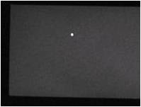
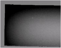
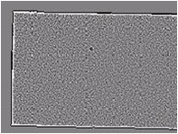
| + | Application of the Laplacian removes substantial inhomogeniety in the field map in both phantoms as shown in Fig. 3 (Rectangular phantom) and Fig. 4 (Cylindrical phantom). Rectangular phantom: mean estimated susceptibility values for water and Magnevist were -9.049 and 0.6273 ppm, with true values of -9.050 and 0.6270 ppm. Cylindrical phantom: the estimated susceptibility map allowed different concentrations of Magnevist to be clearly identified and reasonable estimates were obtained in the presence of significant noise and bias due to external field effects. | ||
{| | {| | ||
| − | |[[File: | + | |[[File:Box mag.jpg|thumb|300|Fig 3a. Magnitude Image]] |
| − | + | |[[File:Box fmap.png|thumb|300|Fig 3b. Field map]] | |
| − | map | + | |[[File:Box fmap lp.png|thumb|300|Fig 3c. Laplacian of the Field]] |
| − | + | |[[File:Box susc.png|thumb|300|Fig 3d. Estimated Susceptibility (ppm)]] | |
| − | |||
| − | |||
| − | |||
| − | |||
| − | |||
| − | |||
|} | |} | ||
| − | |||
{| | {| | ||
| − | |[[File: | + | |[[File:Cyl mag.png|thumb|300|Fig 4a. Magnitude Image]] |
| + | |[[File:Cyl fmap.png|thumb|300|Fig 4b. Field map]] | ||
| + | |[[File:Cyl fmap lp.png|thumb|300|Fig 4c. Laplacian of the Field]] | ||
| + | |[[File:Cyl susc.png|thumb|300|Fig 4d. Estimated Susceptibility (ppm)]] | ||
| + | |[[File:Susc plot2.png|thumb|100|Fig 4e. Estimated vs. True mean susceptibility values for each tube (ppm)]] | ||
|} | |} | ||
| + | = Future Directions = | ||
| + | |||
| + | Future work will focus on quantifying magnetic susceptibility and iron content in the brain. Further development of the method described above has generated the preliminary results shown below in Fig 5. | ||
{| | {| | ||
| − | |[[File: | + | |[[File:Miccai fig1 crop.png|thumb|600px|Fig 5. The field map (left), laplacian of the field (center) and estimated susceptibility map (right) for a young healthy subject is shown. Taking the Laplacian of the fieldmap successfully eliminates the substantial biasfields in the observed field. The estimated susceptibility map shares similar high frequency structure with the Laplacian of the observed field while low frequency structure is preserved by additional modeling constraints.]] |
| − | | | ||
| − | |||
|} | |} | ||
| + | |||
| + | = References = | ||
| + | |||
| + | 1. Zecca L, et al. Nat Rev Neurosci, 5:863{73, Nov 2004. | ||
| + | |||
| + | 2. Lustig M,et al. MRM. 2007. 58(6):1182. | ||
| + | |||
| + | 3. Jenkinson M, et al. MRM. 2004. 52(3):471. | ||
| + | |||
| + | 4. de Rochefort L, et al. MRM.2010. 63(1):194. | ||
| + | |||
| + | 5. Weisskoff RM, et al. MRM. 1992. 24(2):375. | ||
| + | |||
| + | = Key Investigators = | ||
| + | |||
| + | * MIT: Clare Poynton, Elfar Adalsteinsson | ||
| + | * Harvard/BWH: William Wells | ||
| + | * Stanford: Adolf Pfefferbaum, Edith Sullivan | ||
Latest revision as of 19:47, 28 November 2012
Home < Projects:QuantitativeSusceptibilityMappingContents
Introduction
There is increasing evidence that excessive iron deposition in specific regions of the brain is associated with neurodegenerative disorders such as Alzheimer's and Parkinson's disease [1]. The role of iron in the pathogenesis of these diseases remains unknown and is difficult to determine without a non-invasive method to quantify its concentration in-vivo. Since iron is a ferromagnetic substance, changes in iron concentration result in local changes in the magnetic susceptibility of tissue. In magnetic resonance imaging (MRI) experiments, differences in magnetic susceptibility cause perturbations in the local magnetic field, which can be computed from the phase of the MR signal (in a gradient echo sequence, the observed field is proportional to the MR phase).
Description
In MRI, magnetic susceptibility differences cause measurable perturbations in the local magnetic field that can be modeled as the convolution of a dipole-like kernel with the spatial susceptibility distribution. In the Fourier domain, the kernel exhibits zeros at the magic angle, preventing direct inversion of the field map; also, limited observations make the problem ill-posed. The observed data is also corrupted by confounding fields (ie. those from tissue/air interfaces, mis-set shims, and other non-local sources). Previous work has shown that MR images can be successfully reconstructed from under-sampled observations by exploiting the sparsity of in-vivo data under various transforms using methods from compressed sensing [2]. In susceptibility estimation, the forward model results in under-sampling of the data in the Fourier domain, but accurate estimates can be obtained using the Laplacian and L1 norm, which promote sparse solutions while removing external field artifacts. Our variational method for susceptibility estimation is described in Figs. 1-2.
Forward Model (Eq. 1)
The forward model relates the perturbing field to the unknown susceptibility through a local term and convolution of the second z-derivative of the Green’s function of the Laplacian with the unknown susceptibility map [3].
Bias Field Elimination (Eq. 2)
Applying the Laplacian removes non-local phase effects such as shim fields, which are a solution to the Laplace equation.
Objective Function (Eq. 3)
The first term provides regularization, penalizing solutions with large differences in spatial frequency structure relative to the magnitude image. The second term penalizes departures from Eq. 2, by enforcing agreement of high frequency phase effects while eliminating low order bias fields.
Data Acquisition
Cylindrical and rectangular phantoms were made using Magnevist (gadopentetate dimeglumine) solutions of 0.5, 1.0, 2.0, and 3.0 mM corresponding to susceptibility values of 0.15, 0.31, 0.62, and 0.94 ppm [4,5]. Field maps were obtained using a 3D multi-echo GRE sequence on a 3T Siemens Trio MRI.
Results
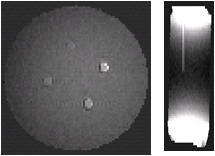
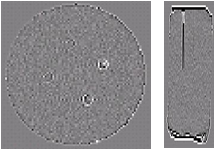
Application of the Laplacian removes substantial inhomogeniety in the field map in both phantoms as shown in Fig. 3 (Rectangular phantom) and Fig. 4 (Cylindrical phantom). Rectangular phantom: mean estimated susceptibility values for water and Magnevist were -9.049 and 0.6273 ppm, with true values of -9.050 and 0.6270 ppm. Cylindrical phantom: the estimated susceptibility map allowed different concentrations of Magnevist to be clearly identified and reasonable estimates were obtained in the presence of significant noise and bias due to external field effects.
Future Directions
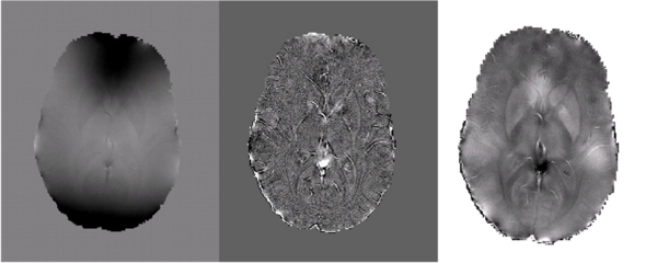
Future work will focus on quantifying magnetic susceptibility and iron content in the brain. Further development of the method described above has generated the preliminary results shown below in Fig 5.
References
1. Zecca L, et al. Nat Rev Neurosci, 5:863{73, Nov 2004.
2. Lustig M,et al. MRM. 2007. 58(6):1182.
3. Jenkinson M, et al. MRM. 2004. 52(3):471.
4. de Rochefort L, et al. MRM.2010. 63(1):194.
5. Weisskoff RM, et al. MRM. 1992. 24(2):375.
Key Investigators
- MIT: Clare Poynton, Elfar Adalsteinsson
- Harvard/BWH: William Wells
- Stanford: Adolf Pfefferbaum, Edith Sullivan

