|
|
| (61 intermediate revisions by 2 users not shown) |
| Line 1: |
Line 1: |
| − | Quantifying magnetic susceptibility in the brain from the phase of the MR signal
| + | = Introduction = |
| − | provides a non-invasive means for measuring the accumulation
| |
| − | of iron believed to occur with aging and neurodegenerative disease.
| |
| − | Phase observations from local susceptibility distributions,
| |
| − | however, are corrupted by external biasfields, which
| |
| − | may be identical to the sources of interest. Furthermore,
| |
| − | limited observations of the phase makes the inversion ill-posed. We
| |
| − | describe a variational approach to susceptibility estimation that
| |
| − | incorporates a tissue-air atlas to resolve ambiguity in the forward model, while eliminating additional biasfields
| |
| − | through application of the Laplacian. Results show qualitative improvement
| |
| − | over two methods commonly used to infer underlying
| |
| − | susceptibility values, and quantitative susceptibility estimates
| |
| − | show better correlation with postmortem iron concentrations than
| |
| − | competing methods.
| |
| − | | |
| − | = Description = | |
| | | | |
| | There is increasing evidence that excessive iron deposition in specific regions | | There is increasing evidence that excessive iron deposition in specific regions |
| Line 26: |
Line 11: |
| | can be computed from the phase of the MR signal (in a gradient echo sequence, the observed field is proportional to the MR phase). | | can be computed from the phase of the MR signal (in a gradient echo sequence, the observed field is proportional to the MR phase). |
| | | | |
| | + | = Description = |
| | + | |
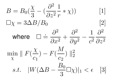
| | + | In MRI, magnetic susceptibility differences cause measurable perturbations in the local magnetic field that can be modeled as the convolution of a dipole-like kernel with the spatial susceptibility distribution. In the Fourier domain, the kernel exhibits zeros at the magic angle, preventing direct inversion of the field map; also, limited observations make the problem ill-posed. The observed data is also corrupted by confounding fields (ie. those from tissue/air interfaces, mis-set shims, and other non-local sources). Previous work has shown that MR images can be successfully reconstructed from under-sampled observations by exploiting the sparsity of in-vivo data under various transforms using methods from compressed sensing [2]. In susceptibility estimation, the forward model results in under-sampling of the data in the Fourier domain, but accurate estimates can be obtained using the Laplacian and L1 norm, which promote sparse solutions while removing external field artifacts. Our variational method for susceptibility estimation is described in Figs. 1-2. |
| | + | |
| | + | {| |
| | + | |[[File:Namic wiki fig1.png|thumb|400px|Fig 1. Relevant notation]] |
| | + | |} |
| | | | |
| − | The field perturbations caused by magnetic susceptibility differences can be
| + | {| |
| − | modeled as the convolution of a dipole-like kernel with the spatial susceptibility
| + | |[[File:Latex pdf zoomed to paint equations.PNG|thumb|400px|Fig 2. Applying the Laplacian to the forward model in [1] eliminates non-local phase artifacts to give [2]. The first term in [3] provides regularization, penalizing large differences in spatial frequency relative to Magnitude data, while the second penalizes departures from [2], enforcing agreement of high frequency phase effects.]] |
| − | distribution. In the Fourier domain, the kernel exhibits zeros at the magic angle,
| + | |} |
| − | preventing direct inversion of the fieldmap [3]. Critically, limited observations of
| |
| − | the field make the problem ill-posed. The observed data is also corrupted by
| |
| − | confounding biasfields (ie. those from tissue-air interfaces, mis-set shims, and other
| |
| − | non-local sources). Eliminating these fields is critical for accurate susceptibility
| |
| − | estimation since they corrupt the phase contributions from local susceptibility
| |
| − | sources.
| |
| | | | |
| | + | == Forward Model (Eq. 1) == |
| | | | |
| − | In general, methods that rely heavily on agreement between observed and
| + | The forward model relates the perturbing field to the unknown susceptibility through a local term and convolution of the second z-derivative of the Green’s function of the Laplacian with the unknown susceptibility map [3]. |
| − | predicted field values computed using kernel-based forward models [2, 3, 6] are
| |
| − | inherently limited since they cannot distinguish between low frequency biasfields
| |
| − | and susceptibility distributions that are eigenfunctions of the model. Examples
| |
| − | of such distributions include constant, linear, and quadratic functions of
| |
| − | susceptibility along the main field (ie. 'z') direction. Applying the forward model to
| |
| − | these distributions results in predicted fields that are proportional to the local
| |
| − | susceptibility sources, but also identical in form to non-local biasfields (ie. those | |
| − | produced by a z-shim). Therefore, removing all low frequency fields prior to
| |
| − | susceptibility estimation will eliminate the biasfield as well as fields due to the
| |
| − | sources of interest, potentially preventing accurate calculation of the underlying
| |
| − | susceptibility values. In contrast, inadequate removal of the biasfield may result
| |
| − | in the estimation of artifactual susceptibility eigenfunctions in areas where the
| |
| − | biasfield is strong, such as regions adjacent to tissue-air interfaces. This suggests
| |
| − | that additional information such as boundary conditions or priors may be necessary to
| |
| − | regularize an incomplete forward model and prevent the mis-estimation
| |
| − | of low frequency biasfields.
| |
| | | | |
| | + | == Bias Field Elimination (Eq. 2) == |
| | | | |
| − | We present a variational approach for Atlas-based Susceptibility Mapping
| + | Applying the Laplacian removes non-local phase effects such as shim fields, which are a solution to the Laplace equation. |
| − | (ASM) that performs simultaneous susceptibility estimation and biasfield
| |
| − | removal using the Laplacian operator and a tissue-air susceptibility atlas. In [7,
| |
| − | 8, 6] it was shown that applying the Laplacian to the observed field eliminates
| |
| − | non-local biasfields due to mis-set shims and remote susceptibility
| |
| − | distributions (ie. the neck/chest).
| |
| − | In this method, large deviations from the susceptibility atlas are penalized,
| |
| − | discouraging the estimation of artifactual susceptibility eigenfunctions in regions near
| |
| − | tissue-air boundaries where the Laplacian may not be sufficient to eliminate the
| |
| − | contribution of non-local sources and substantial signal loss corrupts the observed field.
| |
| − | Agreement of predicted and observed fields
| |
| − | within the brain is also enforced, but deviations in estimated susceptibility values outside the
| |
| − | brain are not penalized, allowing values at the boundary to vary from
| |
| − | the atlas-based prior to account for unmodeled external field sources (ie. shims). | |
| | | | |
| − | = Results = | + | == Objective Function (Eq. 3) == |
| | + | |
| | + | The first term provides regularization, penalizing solutions with large differences in spatial frequency structure relative to the magnitude image. |
| | + | The second term penalizes departures from Eq. 2, by enforcing agreement of high frequency phase effects while eliminating low order bias fields. |
| | | | |
| − | The method is evaluated by comparison of susceptibility maps estimated using ASM to results from Susceptibility Weighted Imaging (SWI) and Field Dependent Relaxation Imaging (FDRI). In SWI, a filtered phase map is obtained by applying a high-pass filter to the phase data, and the resulting SWI map is commonly used as a proxy for susceptibility.
| + | == Data Acquisition == |
| − | While SWI has shown some correlation with magnetic susceptibility differences
| |
| − | due to iron and other sources, the phase maps it yields are only an indirect
| |
| − | measure of susceptibility due to the non-local effects of the convolution kernel.
| |
| − | In addition, the filtering process may remove some low frequency fields due to
| |
| − | sources inside the brain. In FDRI, R2 maps are acquired at two different field strengths (ie. 1.5
| |
| − | and 3 Tesla) and the difference in R2 divided by the difference in field strength
| |
| − | gives the FDRI. The mean FDRI in several regions of interest was previously compared
| |
| − | to the mean iron concentration obtained from postmortem analysis and showed
| |
| − | stronger correlation with iron content than the SWI maps computed for the same
| |
| − | subjects. Obtaining FDRI measurements would be impractical for most studies,
| |
| − | however, since it requires images to be collected on two separate scanners.
| |
| − | In this work, quantitative results are obtained by comparison of mean susceptibility
| |
| − | values in the thalamus (TH), caudate (CD), putamen (PT)
| |
| − | and globus pallidus (GP) to corresponding results from SWI, FDRI and postmortem data.
| |
| | | | |
| | + | Cylindrical and rectangular phantoms were made using Magnevist (gadopentetate dimeglumine) solutions of 0.5, 1.0, 2.0, and 3.0 mM corresponding to susceptibility values of 0.15, 0.31, 0.62, and 0.94 ppm [4,5]. Field maps were obtained using a 3D multi-echo GRE sequence on a 3T Siemens Trio MRI. |
| | | | |
| − | ASM results for a young subject are shown in Fig. 1. Column 1 shows the T1
| + | = Results = |
| − | structural (row 1) and acquired fieldmap (row 2). Application of the Laplacian
| |
| − | to the field map (row 2, column 2) removes substantial B0 inhomogeneities that
| |
| − | bias the observed field. The susceptibility atlas is shown in row 1, column 2
| |
| − | and estimated external sources are shown in row 1, column 3. The estimated
| |
| − | susceptibility map (row2, column 3) shares high frequency structure with the
| |
| − | Laplacian of the observed field, while low frequency structure is preserved by
| |
| − | enforcing agreement with additional information provided by the atlas-based
| |
| − | prior and observed field.
| |
| | | | |
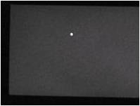
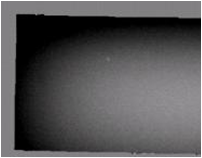
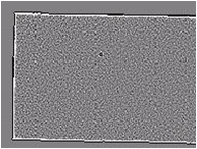
| | + | Application of the Laplacian removes substantial inhomogeniety in the field map in both phantoms as shown in Fig. 3 (Rectangular phantom) and Fig. 4 (Cylindrical phantom). Rectangular phantom: mean estimated susceptibility values for water and Magnevist were -9.049 and 0.6273 ppm, with true values of -9.050 and 0.6270 ppm. Cylindrical phantom: the estimated susceptibility map allowed different concentrations of Magnevist to be clearly identified and reasonable estimates were obtained in the presence of significant noise and bias due to external field effects. |
| | | | |
| | {| | | {| |
| − | |[[File:Fig1 compound lighter v2.png|400px|thumb|Fig. 1: ASM Results. | + | |[[File:Box mag.jpg|thumb|300|Fig 3a. Magnitude Image]] |
| − | The first column shows the T1 structural image (row 1) and field
| + | |[[File:Box fmap.png|thumb|300|Fig 3b. Field map]] |
| − | map (row 2) with substantial inhomogeneity that was obtained from a young subject. | + | |[[File:Box fmap lp.png|thumb|300|Fig 3c. Laplacian of the Field]] |
| − | Column 2 shows the susceptibility atlas (row 1), in which voxels take continuous values
| + | |[[File:Box susc.png|thumb|300|Fig 3d. Estimated Susceptibility (ppm)]] |
| − | between [0,1] corresponding to susceptibility values between air and tissue. Taking
| |
| − | the Laplacian of the fieldmap successfully eliminates biasfields (row 2, column 2).
| |
| − | Estimates of external sources are shown in row 1, column 3. The estimated susceptibility
| |
| − | map (row 2, column 3) shares similar high frequency structure with the Laplacian of
| |
| − | the observed field while low frequency structure is preserved by enforcing agreement
| |
| − | with the atlas and observed field.]]
| |
| | |} | | |} |
| | | | |
| − | Fig. 2 shows results from FDRI (row 1, column 2), SWI (row 1,column 3), | + | {| |
| − | ASM for a young subject (row 2, column 3), and ASM results for 2 elderly
| + | |[[File:Cyl mag.png|thumb|300|Fig 4a. Magnitude Image]] |
| − | subjects (row 2, columns 1,2). The FDRI shows strong constrast between the
| + | |[[File:Cyl fmap.png|thumb|300|Fig 4b. Field map]] |
| − | ROIs and surrounding tissue, but less high frequency structure than the SWI.
| + | |[[File:Cyl fmap lp.png|thumb|300|Fig 4c. Laplacian of the Field]] |
| − | The SWI retains high frequency phase effects, but indiscriminately removes low
| + | |[[File:Cyl susc.png|thumb|300|Fig 4d. Estimated Susceptibility (ppm)]] |
| − | order fields from both internal and external sources, resulting in artifactual low
| + | |[[File:Susc plot2.png|thumb|100|Fig 4e. Estimated vs. True mean susceptibility values for each tube (ppm)]] |
| − | frequency structure. The ASM method accurately preserves the high frequency
| + | |} |
| − | phase effects seen in SWI while showing improved estimation of low order susceptibility
| |
| − | distributions. In addition, ASM provides direct estimates of susceptibility
| |
| − | values rather than filtered phase values that serve as proxies for susceptibility.
| |
| | | | |
| | + | = Future Directions = |
| | + | |
| | + | Future work will focus on quantifying magnetic susceptibility and iron content in the brain. Further development of the method described above has generated the preliminary results shown below in Fig 5. |
| | | | |
| | {| | | {| |
| − | |[[File:Fig2 compound lighter.png|400px|thumb|Fig. 2: Comparison of Results. | + | |[[File:Miccai fig1 crop.png|thumb|600px|Fig 5. The field map (left), laplacian of the field (center) and estimated susceptibility map (right) for a young healthy subject is shown. Taking the Laplacian of the fieldmap successfully eliminates the substantial biasfields in the observed field. The estimated susceptibility map shares similar high frequency structure with the Laplacian of the observed field while low frequency structure is preserved by additional modeling constraints.]] |
| − | Row 1 shows the T1 structural image (column 1), FDRI
| |
| − | (column 2) and SWI (column 3) results for a young subject. ASM results are shown in | |
| − | row 2 for young (column 3) and elderly (columns 1,2) subjects. The FDRI shows strong
| |
| − | constrast between ROIs and adjacent tissue, but less high frequency structure than
| |
| − | the SWI. The SWI retains high frequency phase effects, but indiscriminately removes | |
| − | low order fields from both internal and external sources, resulting in artifactual low
| |
| − | frequency structure. ASM accurately preserves the high frequency structure seen in
| |
| − | SWI while showing improved estimation of low order susceptibility distributions.]]
| |
| | |} | | |} |
| | | | |
| | + | = References = |
| | | | |
| − | Quantitative results from ASM and previously reported results from FDRI
| + | 1. Zecca L, et al. Nat Rev Neurosci, 5:863{73, Nov 2004. |
| − | and SWI for 12 elderly subjects are shown in Fig. 3. The mean
| |
| − | susceptibility values (relative to tissue susceptibility) in each ROI from all elderly subjects are plotted
| |
| − | against the corresponding iron concentrations from postmortem analysis (only
| |
| − | the mean and SD in each ROI was reported in [17]). ASM shows a high
| |
| − | correlation with postmortem values, which is comparable to that seen in FDRI and
| |
| − | substantially better than the correlation between phase and iron concentration
| |
| − | obtained with SWI. In addition, for the structures that we analyzed, ASM results
| |
| − | compare favorably to the correlation between postmortem iron and
| |
| − | susceptibility estimates in corresponding ROIs computed from multi-angle acquisitions [6].
| |
| | | | |
| | + | 2. Lustig M,et al. MRM. 2007. 58(6):1182. |
| | | | |
| − | {|
| + | 3. Jenkinson M, et al. MRM. 2004. 52(3):471. |
| − | |[[File:Fig3 elderly compound.png|800px|thumb|Fig. 3: Quantitative Results. The Mean +/- SD iron concentration
| + | |
| − | (mg/100g fresh weight)
| + | 4. de Rochefort L, et al. MRM.2010. 63(1):194. |
| − | in each ROI determined from postmortem analysis [17] is plotted on the x-axis. The y-
| + | |
| − | axes show the Mean +/- SD FDRI (s^{-1}/Tesla), Mean +/- SD SWI (radians), and Mean +/- SD
| + | 5. Weisskoff RM, et al. MRM. 1992. 24(2):375. |
| − | ASM susceptibility (ppm). Mean susceptibility values from ASM show a high
| |
| − | correlation with the postmortem data, which agrees well with previous results from FDRI
| |
| − | and shows improvement over SWI values reported for the same data [5].]]
| |
| − | |}
| |
| | | | |
| | = Key Investigators = | | = Key Investigators = |
| | | | |
| − | * MIT: Clare Poynton, Elfar Adalsteinsson, Polina Golland | + | * MIT: Clare Poynton, Elfar Adalsteinsson |
| − | * BWH/Harvard: William Wells | + | * Harvard/BWH: William Wells |
| | * Stanford: Adolf Pfefferbaum, Edith Sullivan | | * Stanford: Adolf Pfefferbaum, Edith Sullivan |
Introduction
There is increasing evidence that excessive iron deposition in specific regions
of the brain is associated with neurodegenerative disorders such as Alzheimer's
and Parkinson's disease [1]. The role of iron in the pathogenesis of these diseases
remains unknown and is difficult to determine without a non-invasive method
to quantify its concentration in-vivo. Since iron is a ferromagnetic substance,
changes in iron concentration result in local changes in the magnetic susceptibility of tissue.
In magnetic resonance imaging (MRI) experiments, differences
in magnetic susceptibility cause perturbations in the local magnetic field, which
can be computed from the phase of the MR signal (in a gradient echo sequence, the observed field is proportional to the MR phase).
Description
In MRI, magnetic susceptibility differences cause measurable perturbations in the local magnetic field that can be modeled as the convolution of a dipole-like kernel with the spatial susceptibility distribution. In the Fourier domain, the kernel exhibits zeros at the magic angle, preventing direct inversion of the field map; also, limited observations make the problem ill-posed. The observed data is also corrupted by confounding fields (ie. those from tissue/air interfaces, mis-set shims, and other non-local sources). Previous work has shown that MR images can be successfully reconstructed from under-sampled observations by exploiting the sparsity of in-vivo data under various transforms using methods from compressed sensing [2]. In susceptibility estimation, the forward model results in under-sampling of the data in the Fourier domain, but accurate estimates can be obtained using the Laplacian and L1 norm, which promote sparse solutions while removing external field artifacts. Our variational method for susceptibility estimation is described in Figs. 1-2.
 Fig 2. Applying the Laplacian to the forward model in [1] eliminates non-local phase artifacts to give [2]. The first term in [3] provides regularization, penalizing large differences in spatial frequency relative to Magnitude data, while the second penalizes departures from [2], enforcing agreement of high frequency phase effects. |
Forward Model (Eq. 1)
The forward model relates the perturbing field to the unknown susceptibility through a local term and convolution of the second z-derivative of the Green’s function of the Laplacian with the unknown susceptibility map [3].
Bias Field Elimination (Eq. 2)
Applying the Laplacian removes non-local phase effects such as shim fields, which are a solution to the Laplace equation.
Objective Function (Eq. 3)
The first term provides regularization, penalizing solutions with large differences in spatial frequency structure relative to the magnitude image.
The second term penalizes departures from Eq. 2, by enforcing agreement of high frequency phase effects while eliminating low order bias fields.
Data Acquisition
Cylindrical and rectangular phantoms were made using Magnevist (gadopentetate dimeglumine) solutions of 0.5, 1.0, 2.0, and 3.0 mM corresponding to susceptibility values of 0.15, 0.31, 0.62, and 0.94 ppm [4,5]. Field maps were obtained using a 3D multi-echo GRE sequence on a 3T Siemens Trio MRI.
Results
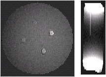
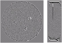
Application of the Laplacian removes substantial inhomogeniety in the field map in both phantoms as shown in Fig. 3 (Rectangular phantom) and Fig. 4 (Cylindrical phantom). Rectangular phantom: mean estimated susceptibility values for water and Magnevist were -9.049 and 0.6273 ppm, with true values of -9.050 and 0.6270 ppm. Cylindrical phantom: the estimated susceptibility map allowed different concentrations of Magnevist to be clearly identified and reasonable estimates were obtained in the presence of significant noise and bias due to external field effects.
|
|
|
 Fig 3c. Laplacian of the Field |
 Fig 3d. Estimated Susceptibility (ppm) |
|
|
|
 Fig 4c. Laplacian of the Field |
 Fig 4d. Estimated Susceptibility (ppm) |
 Fig 4e. Estimated vs. True mean susceptibility values for each tube (ppm) |
Future Directions
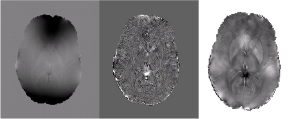
Future work will focus on quantifying magnetic susceptibility and iron content in the brain. Further development of the method described above has generated the preliminary results shown below in Fig 5.
 Fig 5. The field map (left), laplacian of the field (center) and estimated susceptibility map (right) for a young healthy subject is shown. Taking the Laplacian of the fieldmap successfully eliminates the substantial biasfields in the observed field. The estimated susceptibility map shares similar high frequency structure with the Laplacian of the observed field while low frequency structure is preserved by additional modeling constraints. |
References
1. Zecca L, et al. Nat Rev Neurosci, 5:863{73, Nov 2004.
2. Lustig M,et al. MRM. 2007. 58(6):1182.
3. Jenkinson M, et al. MRM. 2004. 52(3):471.
4. de Rochefort L, et al. MRM.2010. 63(1):194.
5. Weisskoff RM, et al. MRM. 1992. 24(2):375.
Key Investigators
- MIT: Clare Poynton, Elfar Adalsteinsson
- Harvard/BWH: William Wells
- Stanford: Adolf Pfefferbaum, Edith Sullivan

