Difference between revisions of "Projects:fMRIDetection"
m (Update from Wiki) |
|||
| (21 intermediate revisions by 6 users not shown) | |||
| Line 1: | Line 1: | ||
| − | = | + | Back to [[NA-MIC_Internal_Collaborations:fMRIAnalysis|NA-MIC_Collaborations]], [[Algorithm:MIT|MIT Algorithms]], [[DBP1:Harvard|Harvard DBP1]] |
| + | __NOTOC__ | ||
| + | = fMRI Detection = | ||
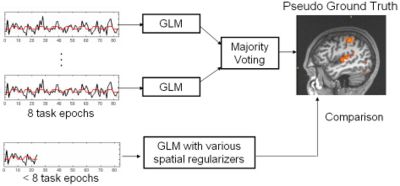
Validation is known as one of the most challenging problem in fMRI analysis since the ground truth activation is unknown. In this work, we evaluate the proposed fMRI analysis methods with respect to their ability to detect activations from reduced-length time courses. The following flow chart depicts our evaluation process. We compare the detection results, obtained from partial-length time courses, to the pseudo ground truth activation map, created by majority voting of the GLM detection results from four full-length sessions (all 17 epochs) in fMRI experiments for the same subject. No smoothing is performed while creating the pseudo ground truth activation maps. | Validation is known as one of the most challenging problem in fMRI analysis since the ground truth activation is unknown. In this work, we evaluate the proposed fMRI analysis methods with respect to their ability to detect activations from reduced-length time courses. The following flow chart depicts our evaluation process. We compare the detection results, obtained from partial-length time courses, to the pseudo ground truth activation map, created by majority voting of the GLM detection results from four full-length sessions (all 17 epochs) in fMRI experiments for the same subject. No smoothing is performed while creating the pseudo ground truth activation maps. | ||
| − | + | ||
| + | [[Image:FMRIEvaluationchart.jpg|thumb|center|400px|This flow chart outlines the validation procedure using real fMRI data.]] | ||
Data across runs and across subjects yields similar results in our comparison experiments of the detectors. We present the results in coronal view for one subject across all detectors in the following figures | Data across runs and across subjects yields similar results in our comparison experiments of the detectors. We present the results in coronal view for one subject across all detectors in the following figures | ||
| − | + | {| | |
| + | |[[Image:Gt_sm007ep3_Sn36.tif|thumb|152px|Pseudo Ground truth activation]] | ||
| + | |[[Image:Glm_sm007ep3_Sn36.tif|thumb|152px|Detection result without spatial regularization]] | ||
| + | |[[Image:Gau_sm007ep3_Sn36.tif|thumb|152px|Detection result with Gaussian smoothing]] | ||
| + | |[[Image:Mf_sm007ep3_Sn36.tif|thumb|152px|Detection result with MRF spatial regularization]] | ||
| + | |[[Image:Mfseg_sm007ep3_Sn36.tif|thumb|152px|Detection result with anatomically-guided MRF spatial regularization]] | ||
| + | |} | ||
Without spatial regularization, the GLM detector's activation map is more fragmented due to loss in statistical power from reducing the length of the signals. The other two images illustrate the results of applying GLM with the MRF priors, as well as its anatomically-guided version. MRF regularization is able to capture activations with elongated spatial structures. This highlights the potential benefit of using the Markov priors in fMRI detection. Furthermore, anatomically-guided MRF produces activations maps that follow closely the highly folded cortical sheet. The MRF model benefits from using anatomical information to remove spurious activations. Our experiments demonstrate that employing anatomically-guided MRF spatial regularization leads to high detection accuracy from time courses of substantially reduced length. | Without spatial regularization, the GLM detector's activation map is more fragmented due to loss in statistical power from reducing the length of the signals. The other two images illustrate the results of applying GLM with the MRF priors, as well as its anatomically-guided version. MRF regularization is able to capture activations with elongated spatial structures. This highlights the potential benefit of using the Markov priors in fMRI detection. Furthermore, anatomically-guided MRF produces activations maps that follow closely the highly folded cortical sheet. The MRF model benefits from using anatomical information to remove spurious activations. Our experiments demonstrate that employing anatomically-guided MRF spatial regularization leads to high detection accuracy from time courses of substantially reduced length. | ||
| Line 13: | Line 22: | ||
<br /> | <br /> | ||
| − | = | + | = Description = |
| − | |||
We study Markov Random Fields (MRF) as spatial smoothing priors in fMRI detection. In this work, we investigate fast approximate inference algorithms for using MRFs in fMRI detection, propose a novel way to incorporate anatomical information into the detection framework, validate the methods through ROC analysis on simulated data and demonstrate their application in a real fMRI study. The following figures illustrate the detection results from phantom data by showing one axial slice of the estimated activation map using our proposed methods. | We study Markov Random Fields (MRF) as spatial smoothing priors in fMRI detection. In this work, we investigate fast approximate inference algorithms for using MRFs in fMRI detection, propose a novel way to incorporate anatomical information into the detection framework, validate the methods through ROC analysis on simulated data and demonstrate their application in a real fMRI study. The following figures illustrate the detection results from phantom data by showing one axial slice of the estimated activation map using our proposed methods. | ||
| − | + | {| | |
| + | |[[Image:Pattern10.tif|thumb|150px|Ground truth activation]] | ||
| + | |[[Image:Glm_p10n0.tif|thumb|150px|Detection result without spatial regularization]] | ||
| + | |[[Image:Gau_p10n0.tif|thumb|150px|Detection result with Gaussian smoothing]] | ||
| + | |[[Image:Mf_p10n0.tif|thumb|150px|Detection result with MRF spatial regularization]] | ||
| + | |[[Image:Mfseg_p10n0.tif|thumb|150px|Detection result with anatomically-guided MRF spatial regularization]] | ||
| + | |} | ||
The detection results are obtained with thresholding at 0.5% false positive rate. Yellow pixels indicate true positve, red pixels indicate false positve, and green pixels indicate false negative. | The detection results are obtained with thresholding at 0.5% false positive rate. Yellow pixels indicate true positve, red pixels indicate false positve, and green pixels indicate false negative. | ||
| Line 25: | Line 39: | ||
<br /> | <br /> | ||
| − | + | ''Implementation'' | |
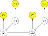
<br /> Cosman [1] demonstrated the potential benefit of using binary MRF as a spatial regularization for fMRI detection. With binary states, exact solution can be obtained in polynomial time. However, if one wants to go beyond binary states (e.g., treating positively and negatively activated voxels differently), the problem of estimating the optimal activation states becomes intractable and approximation algorithms must be used. Our work begins with adopting the Mean Field solver for approximate MRF solution. The following graph depicts the corresponding graphical model. You can find detialed derivation regarding Mean Field solver in [2]. In our experiments, the Mean Field algorithm produced results comparable to those of the exact solver while reducing computation time by one to two orders of magnitude. | <br /> Cosman [1] demonstrated the potential benefit of using binary MRF as a spatial regularization for fMRI detection. With binary states, exact solution can be obtained in polynomial time. However, if one wants to go beyond binary states (e.g., treating positively and negatively activated voxels differently), the problem of estimating the optimal activation states becomes intractable and approximation algorithms must be used. Our work begins with adopting the Mean Field solver for approximate MRF solution. The following graph depicts the corresponding graphical model. You can find detialed derivation regarding Mean Field solver in [2]. In our experiments, the Mean Field algorithm produced results comparable to those of the exact solver while reducing computation time by one to two orders of magnitude. | ||
| − | + | [[Image:MRFnoSegM.fig2ps.tmp.jpg|thumb|left|200px||Graphical model for MRF. Xi and Zi denote activation state and voxel-by-voxel fMRI statistics of voxel i, respectively. Xi is the hidden variable, while Zi is the noisy observation.]] | |
| + | |||
| + | <br clear="all"/> | ||
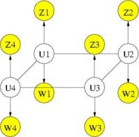
<br /> We further refine MRF spatial regularization by incorporating anatomical information. Similarly to segmentation, where a probabilistic atlas serves as a spatially varying prior on the tissue types, the anatomical information can provide a prior on the activation map. The following figure illustrates the graphical model of the MRF with anatomical information. Intuitively speaking, we want the prior to reflect the fact that activation is much more likely to occur in gray matter than in white matter, and not at all in cerebrospinal fluid (CSF) or bone. In addition, the spatial coherency of activation is strong within each tissue and not across tissue boundaries. | <br /> We further refine MRF spatial regularization by incorporating anatomical information. Similarly to segmentation, where a probabilistic atlas serves as a spatially varying prior on the tissue types, the anatomical information can provide a prior on the activation map. The following figure illustrates the graphical model of the MRF with anatomical information. Intuitively speaking, we want the prior to reflect the fact that activation is much more likely to occur in gray matter than in white matter, and not at all in cerebrospinal fluid (CSF) or bone. In addition, the spatial coherency of activation is strong within each tissue and not across tissue boundaries. | ||
| − | + | [[Image:MRFSegM2.fig2ps.tmp.jpg|thumb|left|200px|Graphical model for MRF with anatomical information. Wi denotes (potentially noisy) segmentation label of voxel i. U_i is combination of activation state and true tissue type of voxel i. Wi and Zi are noisy obervations, and Ui is the hidden variable.]] | |
| + | |||
| + | <br clear="all"/> | ||
<br /> In our experiments, we compared our proposed spatial regularization methods: MRF solved by Mean Field algorithm and MRF with anatomical information, with most common spatial regulariation method: Gaussian smoothing. We found that MRF's detection rate is higher than Guassian smoothing's results when the signal to noise ratio (SNR) of the date is relatively high. Incorporating anatomical information to either MRF or Gaussian smoothing can further improve their performance disregarding the SNR level. | <br /> In our experiments, we compared our proposed spatial regularization methods: MRF solved by Mean Field algorithm and MRF with anatomical information, with most common spatial regulariation method: Gaussian smoothing. We found that MRF's detection rate is higher than Guassian smoothing's results when the signal to noise ratio (SNR) of the date is relatively high. Incorporating anatomical information to either MRF or Gaussian smoothing can further improve their performance disregarding the SNR level. | ||
| − | + | ''Software'' | |
| − | + | MRF/based regularizers and anatomically-guided fMRI detection tools are being integrated into Slicer. | |
| − | |||
| − | * Wanmei Ou, Polina Golland | + | = Key Investigators = |
| + | |||
| + | * MIT: Wanmei Ou, Polina Golland | ||
| + | * Harvard DBP1: Sandy Wells, Wendy Plesniak, Carsten Richter | ||
| + | |||
| − | + | = Publications = | |
| + | ''In Print'' | ||
| − | = | + | * [http://www.na-mic.org/publications/pages/display?search=Projects%3AfMRIDetection&submit=Search&words=all&title=checked&keywords=checked&authors=checked&abstract=checked&sponsors=checked&searchbytag=checked| NA-MIC Publications Database on fMRI Detection and Analysis] |
| − | + | [[Category: fMRI]] [[Category: Slicer]] | |
Latest revision as of 20:20, 11 May 2010
Home < Projects:fMRIDetectionBack to NA-MIC_Collaborations, MIT Algorithms, Harvard DBP1
fMRI Detection
Validation is known as one of the most challenging problem in fMRI analysis since the ground truth activation is unknown. In this work, we evaluate the proposed fMRI analysis methods with respect to their ability to detect activations from reduced-length time courses. The following flow chart depicts our evaluation process. We compare the detection results, obtained from partial-length time courses, to the pseudo ground truth activation map, created by majority voting of the GLM detection results from four full-length sessions (all 17 epochs) in fMRI experiments for the same subject. No smoothing is performed while creating the pseudo ground truth activation maps.
Data across runs and across subjects yields similar results in our comparison experiments of the detectors. We present the results in coronal view for one subject across all detectors in the following figures
| File:Gt sm007ep3 Sn36.tif | File:Glm sm007ep3 Sn36.tif | File:Gau sm007ep3 Sn36.tif | File:Mf sm007ep3 Sn36.tif | File:Mfseg sm007ep3 Sn36.tif |
Without spatial regularization, the GLM detector's activation map is more fragmented due to loss in statistical power from reducing the length of the signals. The other two images illustrate the results of applying GLM with the MRF priors, as well as its anatomically-guided version. MRF regularization is able to capture activations with elongated spatial structures. This highlights the potential benefit of using the Markov priors in fMRI detection. Furthermore, anatomically-guided MRF produces activations maps that follow closely the highly folded cortical sheet. The MRF model benefits from using anatomical information to remove spurious activations. Our experiments demonstrate that employing anatomically-guided MRF spatial regularization leads to high detection accuracy from time courses of substantially reduced length.
Description
We study Markov Random Fields (MRF) as spatial smoothing priors in fMRI detection. In this work, we investigate fast approximate inference algorithms for using MRFs in fMRI detection, propose a novel way to incorporate anatomical information into the detection framework, validate the methods through ROC analysis on simulated data and demonstrate their application in a real fMRI study. The following figures illustrate the detection results from phantom data by showing one axial slice of the estimated activation map using our proposed methods.
| File:Pattern10.tif | File:Glm p10n0.tif | File:Gau p10n0.tif | File:Mf p10n0.tif | File:Mfseg p10n0.tif |
The detection results are obtained with thresholding at 0.5% false positive rate. Yellow pixels indicate true positve, red pixels indicate false positve, and green pixels indicate false negative.
Implementation
Cosman [1] demonstrated the potential benefit of using binary MRF as a spatial regularization for fMRI detection. With binary states, exact solution can be obtained in polynomial time. However, if one wants to go beyond binary states (e.g., treating positively and negatively activated voxels differently), the problem of estimating the optimal activation states becomes intractable and approximation algorithms must be used. Our work begins with adopting the Mean Field solver for approximate MRF solution. The following graph depicts the corresponding graphical model. You can find detialed derivation regarding Mean Field solver in [2]. In our experiments, the Mean Field algorithm produced results comparable to those of the exact solver while reducing computation time by one to two orders of magnitude.
We further refine MRF spatial regularization by incorporating anatomical information. Similarly to segmentation, where a probabilistic atlas serves as a spatially varying prior on the tissue types, the anatomical information can provide a prior on the activation map. The following figure illustrates the graphical model of the MRF with anatomical information. Intuitively speaking, we want the prior to reflect the fact that activation is much more likely to occur in gray matter than in white matter, and not at all in cerebrospinal fluid (CSF) or bone. In addition, the spatial coherency of activation is strong within each tissue and not across tissue boundaries.
In our experiments, we compared our proposed spatial regularization methods: MRF solved by Mean Field algorithm and MRF with anatomical information, with most common spatial regulariation method: Gaussian smoothing. We found that MRF's detection rate is higher than Guassian smoothing's results when the signal to noise ratio (SNR) of the date is relatively high. Incorporating anatomical information to either MRF or Gaussian smoothing can further improve their performance disregarding the SNR level.
Software
MRF/based regularizers and anatomically-guided fMRI detection tools are being integrated into Slicer.
Key Investigators
- MIT: Wanmei Ou, Polina Golland
- Harvard DBP1: Sandy Wells, Wendy Plesniak, Carsten Richter
Publications
In Print


