Difference between revisions of "Projects:fMRIClustering"
| (2 intermediate revisions by 2 users not shown) | |||
| Line 3: | Line 3: | ||
= Improving fMRI Analysis using Supervised and Unsupervised Learning = | = Improving fMRI Analysis using Supervised and Unsupervised Learning = | ||
| − | One of the major goals in the analysis of fMRI data is the detection of | + | One of the major goals in the analysis of fMRI data is the detection of regions of the brain with similar functional behavior. A wide variety of methods including hypothesis-driven statistical tests, supervised, and unsupervised learning methods have been employed to find these networks. In this project, we develop novel learning algorithms that enable more efficient inferences from fMRI measurements. |
| − | = Clustering for the | + | = Clustering for Discovering Structure in the Space of Functional Selectivity = |
| − | + | We are devising clustering algorithms for discovering structure in the functional organization of the high-level visual cortex. It is suggested that there are regions in the visual cortex with high selectivity to certain categories of visual stimuli; we refer to these regions as /functional units/. Currently, the conventional method for detection of these regions is based on statistical tests comparing response of each voxel in the brain to different visual categories to see if it shows considerably higher activation to one category. For example, the well-known FFA (Fusiform Face Area) is the set of voxels which show high activation to face images. We use a model-based clustering approach to the analysis of this type of data as a means to make this analysis automatic and further discover new structures in the high-level visual cortex. | |
| − | + | We formulate a model-based clustering algorithm that simultaneously | |
| − | + | finds a set of activation profiles and their spatial maps from fMRI time courses. We validate | |
| − | + | our method on data from studies of category selectivity in the visual | |
| − | + | cortex, demonstrating good agreement with findings from prior | |
| − | + | hypothesis-driven methods. This hierarchical model enables functional group analysis | |
| − | + | independent of spatial correspondence among subjects. We have also developed a co-clustering extension of this | |
| − | + | algorithm which can simultaneously find a set of clusters of voxels and categories | |
| − | + | of stimuli in experiments with diverse sets of stimulus categories. Our model is nonparametric, learning the numbers of clusters in both domains as well as the cluster parameters. | |
| − | of | ||
| − | |||
| − | the | ||
| − | |||
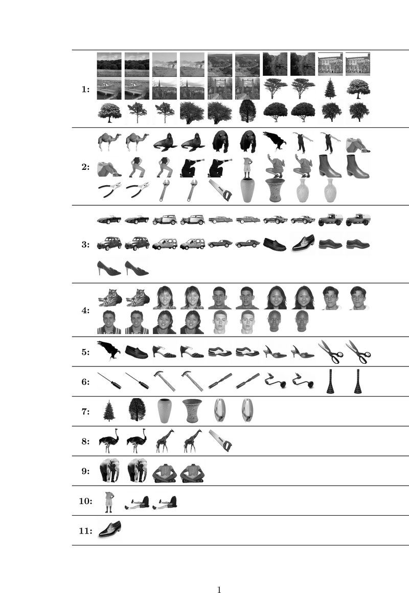
| − | + | Fig. 1 shows the categories learned by our algorithm on a study with 8 subjects. We split trials of each image into two groups of equal size and consider | |
| + | each group as an independent stimulus forming a total of 138 | ||
| + | stimuli. Hence, we can examine the consistency of our stimulus categorization with respect to identical trials. Stimulus pairs | ||
| + | corresponding to the same image are generally assigned to the same | ||
| + | category, confirming the consistency of the resuls across | ||
| + | trials. Category 1 corresponds to the scene images and, interestingly, also includes all images of | ||
| + | trees. This may suggest a high level category structure that is not | ||
| + | merely driven by low level features. Such a structure is even more | ||
| + | evident in the 4th category where images of a tiger that has a large | ||
| + | face join human faces. Some other animals are clustered together with human bodies in categories 2 and | ||
| + | 9. Shoes and cars, which have similar shapes, are clustered together | ||
| + | in category 3 while tools are mainly found in category 6. | ||
| − | |||
| − | + | {| | |
| − | + | |+ '''Fig 1. Categories learned from 8 subjects''' | |
| + | |align="center"|[[Image:Category_singlefile1.png |thumb|800px]] | ||
| + | |} | ||
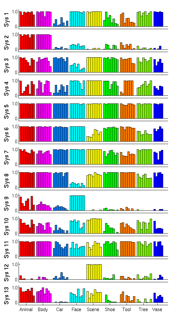
| − | Fig. | + | Fig. 2 shows the cluster centers, or activation profiles, for the first 13 of 25 clusters learned by our method. We see salient category structure in our profiles. For instance, system 1 shows lower responses to cars, shoes, and tools compared to other stimuli. Since the images representing these three categories in our experiment are generally smaller in terms of pixel size, this system appears selective to lower level features (note that the highest probability of activation among shoes corresponds to the largest shoe 3). System 3 and system 8 seem less responsive to faces compared to all other stimuli. |
| − | |||
| − | |||
| − | |||
| − | + | {| | |
| − | + | |+ '''Fig 2. System profiles of posterior probabilities of activation for each system to different stimuli. The bar heights correspond to the posterior probability of activation.''' | |
| − | + | |align="center"|[[Image:Hdpprofs_all_1.png |thumb|800px]] | |
| − | + | |} | |
| − | |||
| − | |||
| − | |||
| − | |||
| − | [[Image: | ||
| − | |||
| − | |||
| − | |||
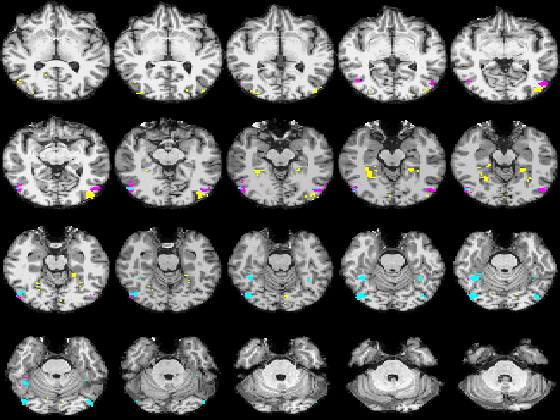
| − | Fig.3 | + | Fig. 3 shows the membership maps for the systems 2, 9, and 12, selective for bodies, faces, and scenes, respectively, which our model learns in a completely unsupervised fashion from the data. For comparison, Fig. 4 shows the significance maps found by applying the conventional confirmatory t-test to the data from the same subject. While significance maps appear to be generally larger than the extent of systems identified by our method, a close inspection reveals that system membership maps include the peak voxels for their corresponding contrasts. |
| − | + | {| | |
| − | + | |+ '''Fig 3. Membership probability maps corresponding to systems 22, 9, and 12, selective respectively for bodies (magenta), scenes (yellow), and faces (cyan) in one subject.''' | |
| − | + | |align="center"|[[Image:Sys_2_9_12_subj1.png |thumb|800px]] | |
| − | [[Image: | + | |} |
| − | |||
| − | |||
| − | |||
{| | {| | ||
| − | |+ '''Fig | + | |+ '''Fig 4. Map representing significance values for three contrasts: bodies-objects (magenta), faces-objects (cyan), and scenes-objects (yellow) in the same subject. Lighter colors correspond to higher significance.''' |
| − | | | + | |align="center"|[[Image:Sys_2_9_12_subj1.png |thumb|800px]] |
|} | |} | ||
| − | ''''' | + | '''''Earlier work''''' |
| − | |||
| − | |||
| − | |||
| − | |||
| − | |||
| − | |||
| − | |||
| − | |||
| − | |||
| − | |||
| − | |||
| − | |||
| − | |||
| − | |||
| − | |||
| − | |||
| − | |||
| − | |||
| − | |||
| − | |||
| − | |||
| − | |||
| − | |||
| − | |||
| − | |||
| − | |||
| − | |||
| − | |||
| − | |||
| − | |||
| − | |||
| − | |||
| − | |||
| − | |||
| − | |||
| − | |||
| − | |||
| − | |||
| − | |||
| − | |||
| − | |||
| − | |||
| − | |||
| − | |||
| − | |||
| − | |||
| − | |||
| − | |||
| − | |||
| − | |||
| − | |||
| − | |||
| − | |||
| − | |||
| − | |||
| − | |||
| − | |||
| − | |||
| − | |||
| − | |||
| − | |||
| − | |||
| − | |||
| − | |||
| − | |||
| − | |||
| − | |||
| − | |||
| − | |||
| − | |||
| − | |||
| − | |||
| − | |||
| − | |||
| − | |||
| − | |||
| − | |||
| − | |||
| − | |||
| − | |||
| − | |||
| − | |||
| − | |||
| − | |||
| − | |||
| − | |||
| − | |||
| − | |||
| − | |||
| − | |||
| − | |||
| − | |||
| − | |||
| − | |||
| − | |||
| − | |||
| − | |||
| − | |||
| − | |||
| − | |||
| − | |||
| − | |||
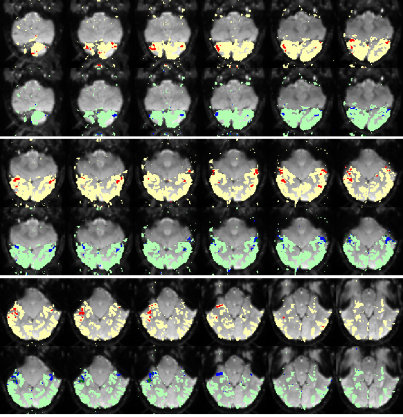
| − | Fig. | + | Fig. 5 compares the map of voxels assigned to a face-selective profile by an earlier version of our algorithm with the t-test's map of voxels with statistically significant (p<0.0001) response to faces when compared with object stimuli. Note that in contrast with the hypothesis testing method, we don't specify the existence of a face-selective region in our algorithm and the algorithm automatically discovers such a profile of activation in the data. |
{| | {| | ||
| − | |+ '''Fig | + | |+ '''Fig 5. Spatial maps of the face selective regions found by the statistical test (red) and our mixture model (dark blue). Maps are presented in alternating rows for comparison. Visually responsive mask of voxels used in our experiment is illustrated in yellow and light blue.''' |
|align="center"|[[Image:mit_fmri_clustering_mapffacompare.PNG |thumb|800px]] | |align="center"|[[Image:mit_fmri_clustering_mapffacompare.PNG |thumb|800px]] | ||
|} | |} | ||
| Line 175: | Line 67: | ||
'''''Hierarchical Model for Exploratory fMRI Analysis without Spatial Normalization''''' | '''''Hierarchical Model for Exploratory fMRI Analysis without Spatial Normalization''''' | ||
| − | Building on the work on the clustering model for the domain specificity, we develop a hierarchical exploratory method for simultaneous parcellation of multisub ect fMRI data into functionally coherent areas. The method is based on a solely functional representation of the fMRI data and a hierarchical probabilistic model that accounts for both inter-subject and intra-subject forms of variability in fMRI response. We employ a Variational Bayes approximation to fit the model to the data. The resulting algorithm finds a functional parcellation of the individual brains along with a set of population-level clusters, establishing correspondence between these two levels. The model eliminates the need for spatial normalization while still enabling us to fuse data from several subjects. We demonstrate the application of our method on the same visual fMRI study as before. Fig. | + | Building on the work on the clustering model for the domain specificity, we develop a hierarchical exploratory method for simultaneous parcellation of multisub ect fMRI data into functionally coherent areas. The method is based on a solely functional representation of the fMRI data and a hierarchical probabilistic model that accounts for both inter-subject and intra-subject forms of variability in fMRI response. We employ a Variational Bayes approximation to fit the model to the data. The resulting algorithm finds a functional parcellation of the individual brains along with a set of population-level clusters, establishing correspondence between these two levels. The model eliminates the need for spatial normalization while still enabling us to fuse data from several subjects. We demonstrate the application of our method on the same visual fMRI study as before. Fig. 6 shows the scene-selective parcel in 2 different subjects. Parcel-level spatial correspondence is evident in the figure between the subjects. |
<table> | <table> | ||
| − | <tr> <th> '''Fig | + | <tr> <th> '''Fig 6. The map of the scene selective parcels in two different subjects. The rough location of the scene-selective areas PPA and TOS, identified by the expert, are shown on the maps by yellow and green circles, respectively.''' |
<tr> | <tr> | ||
<td align="center"> | <td align="center"> | ||
| Line 189: | Line 81: | ||
= Key Investigators = | = Key Investigators = | ||
| − | * MIT: Danial Lashkari, Archana Venkataraman, Ed Vul, Nancy Kanwisher, Polina Golland. | + | * MIT: Danial Lashkari, Archana Venkataraman, Ramesh Sridharan, Ed Vul, Nancy Kanwisher, Polina Golland. |
* Harvard: J. Oh, Marek Kubicki, Carl-Fredrik Westin. | * Harvard: J. Oh, Marek Kubicki, Carl-Fredrik Westin. | ||
Latest revision as of 20:06, 28 November 2012
Home < Projects:fMRIClusteringBack to NA-MIC Collaborations, MIT Algorithms
Improving fMRI Analysis using Supervised and Unsupervised Learning
One of the major goals in the analysis of fMRI data is the detection of regions of the brain with similar functional behavior. A wide variety of methods including hypothesis-driven statistical tests, supervised, and unsupervised learning methods have been employed to find these networks. In this project, we develop novel learning algorithms that enable more efficient inferences from fMRI measurements.
Clustering for Discovering Structure in the Space of Functional Selectivity
We are devising clustering algorithms for discovering structure in the functional organization of the high-level visual cortex. It is suggested that there are regions in the visual cortex with high selectivity to certain categories of visual stimuli; we refer to these regions as /functional units/. Currently, the conventional method for detection of these regions is based on statistical tests comparing response of each voxel in the brain to different visual categories to see if it shows considerably higher activation to one category. For example, the well-known FFA (Fusiform Face Area) is the set of voxels which show high activation to face images. We use a model-based clustering approach to the analysis of this type of data as a means to make this analysis automatic and further discover new structures in the high-level visual cortex.
We formulate a model-based clustering algorithm that simultaneously finds a set of activation profiles and their spatial maps from fMRI time courses. We validate our method on data from studies of category selectivity in the visual cortex, demonstrating good agreement with findings from prior hypothesis-driven methods. This hierarchical model enables functional group analysis independent of spatial correspondence among subjects. We have also developed a co-clustering extension of this algorithm which can simultaneously find a set of clusters of voxels and categories of stimuli in experiments with diverse sets of stimulus categories. Our model is nonparametric, learning the numbers of clusters in both domains as well as the cluster parameters.
Fig. 1 shows the categories learned by our algorithm on a study with 8 subjects. We split trials of each image into two groups of equal size and consider each group as an independent stimulus forming a total of 138 stimuli. Hence, we can examine the consistency of our stimulus categorization with respect to identical trials. Stimulus pairs corresponding to the same image are generally assigned to the same category, confirming the consistency of the resuls across trials. Category 1 corresponds to the scene images and, interestingly, also includes all images of trees. This may suggest a high level category structure that is not merely driven by low level features. Such a structure is even more evident in the 4th category where images of a tiger that has a large face join human faces. Some other animals are clustered together with human bodies in categories 2 and 9. Shoes and cars, which have similar shapes, are clustered together in category 3 while tools are mainly found in category 6.
Fig. 2 shows the cluster centers, or activation profiles, for the first 13 of 25 clusters learned by our method. We see salient category structure in our profiles. For instance, system 1 shows lower responses to cars, shoes, and tools compared to other stimuli. Since the images representing these three categories in our experiment are generally smaller in terms of pixel size, this system appears selective to lower level features (note that the highest probability of activation among shoes corresponds to the largest shoe 3). System 3 and system 8 seem less responsive to faces compared to all other stimuli.
Fig. 3 shows the membership maps for the systems 2, 9, and 12, selective for bodies, faces, and scenes, respectively, which our model learns in a completely unsupervised fashion from the data. For comparison, Fig. 4 shows the significance maps found by applying the conventional confirmatory t-test to the data from the same subject. While significance maps appear to be generally larger than the extent of systems identified by our method, a close inspection reveals that system membership maps include the peak voxels for their corresponding contrasts.
Earlier work
Fig. 5 compares the map of voxels assigned to a face-selective profile by an earlier version of our algorithm with the t-test's map of voxels with statistically significant (p<0.0001) response to faces when compared with object stimuli. Note that in contrast with the hypothesis testing method, we don't specify the existence of a face-selective region in our algorithm and the algorithm automatically discovers such a profile of activation in the data.
Hierarchical Model for Exploratory fMRI Analysis without Spatial Normalization
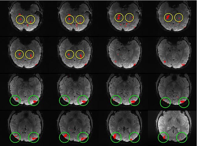
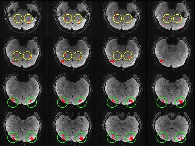
Building on the work on the clustering model for the domain specificity, we develop a hierarchical exploratory method for simultaneous parcellation of multisub ect fMRI data into functionally coherent areas. The method is based on a solely functional representation of the fMRI data and a hierarchical probabilistic model that accounts for both inter-subject and intra-subject forms of variability in fMRI response. We employ a Variational Bayes approximation to fit the model to the data. The resulting algorithm finds a functional parcellation of the individual brains along with a set of population-level clusters, establishing correspondence between these two levels. The model eliminates the need for spatial normalization while still enabling us to fuse data from several subjects. We demonstrate the application of our method on the same visual fMRI study as before. Fig. 6 shows the scene-selective parcel in 2 different subjects. Parcel-level spatial correspondence is evident in the figure between the subjects.
| Fig 6. The map of the scene selective parcels in two different subjects. The rough location of the scene-selective areas PPA and TOS, identified by the expert, are shown on the maps by yellow and green circles, respectively. | |
|---|---|
Key Investigators
- MIT: Danial Lashkari, Archana Venkataraman, Ramesh Sridharan, Ed Vul, Nancy Kanwisher, Polina Golland.
- Harvard: J. Oh, Marek Kubicki, Carl-Fredrik Westin.
Publications
NA-MIC Publications Database on fMRI clustering
Project Week Results: June 2008
