Difference between revisions of "Projects:GroupwiseRegistration"
| Line 74: | Line 74: | ||
| − | where <math>B_l</math> is | + | where <math>B_l</math> is <math>l</math>'th cubic B-spline basis function. <math>(u,v,w)</math> is the distance |
to <math>(x,y,z)</math> from the control point <math>\Phi_{i,j,k}</math> as shown in Figure 2. | to <math>(x,y,z)</math> from the control point <math>\Phi_{i,j,k}</math> as shown in Figure 2. | ||
| Line 98: | Line 98: | ||
First, we perform a global registration with affine transforms. | First, we perform a global registration with affine transforms. | ||
Then, we use affine transforms to initialize a low resolution deformation field | Then, we use affine transforms to initialize a low resolution deformation field | ||
| − | at a grid spacing around | + | at a grid spacing around 32 voxels. |
| − | We increase the resolution of the deformation field to | + | We increase the resolution of the deformation field to 8 voxels |
by using registration results at coarser grids to initialize finer grids. | by using registration results at coarser grids to initialize finer grids. | ||
| Line 116: | Line 116: | ||
We implemented our groupwise registration method in a multi-threaded fashion using Insight Toolkit (ITK) | We implemented our groupwise registration method in a multi-threaded fashion using Insight Toolkit (ITK) | ||
| − | and made the implementation publicly available | + | and made the implementation publicly available. |
We run experiments using a dataset of 50 MR images | We run experiments using a dataset of 50 MR images | ||
with $256\times256\times128$ voxels on a workstation with four CPUs and | with $256\times256\times128$ voxels on a workstation with four CPUs and | ||
Revision as of 23:21, 9 November 2007
Home < Projects:GroupwiseRegistrationBack to NA-MIC_Collaborations, MIT Algorithms
Non-rigid Groupwise Registration
We aim at providing efficient groupwise registration algorithms for population analysis of anatomical structures. Here we extend a previously demonstrated entropy based groupwise registration method to include a free-form deformation model based on B-splines. We provide an efficient implementation using stochastic gradient descents in a multi-resolution setting. We demonstrate the method in application to a set of 50 MRI brain scans and compare the results to a pairwise approach using segmentation labels to evaluate the quality of alignment. Our results indicate that increasing the complexity of the deformation model improves registration accuracy significantly, especially at cortical regions.
Description
We first describe the stack entropy cost function and the B-spline based deformation model. Then we discuss implementation details. Next, we compare groupwise registration to the pairwise method and evaluate both methods using label prediction values.
Objective Function

In order to align all subjects in the population, we consider sum of pixelwise entropies as a joint alignment criterion. The justification for this approach is that if the images are aligned properly, intensity values at corresponding coordinate locations from all the images will form a low entropy distribution. This approach does not require the use of a reference subject; all subjects are simultenously driven to the common tendency of the population.
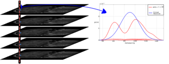
We employ a kernel based density estimation scheme to estimate univariate entropies. Using the entropy measure we obtain a better treatment of transitions between different tissue types, such as gray matter-white matter transitions in the cortical regions where intensity distributions can be bi-modal as shown in Figure 1.
Deformation Model
For the nonrigid deformation model, we define a combined transformation consisting of a global and a local component
- [math] T(\mathbf{x}) = T_{local}({T_{global}(\mathbf{x})}) [/math]
where [math]T_{global}[/math] is a twelve parameter affine transform and [math]T_{local}[/math] is a deformation model based on B-splines.
The free form deformation can be written as the 3-D tensor product of 1-D cubic B-splines.
- [math] T_{local}(\mathbf{x}) = \mathbf{x} + \sum_{l=0}^3\sum_{m=0}^3\sum_{n=0}^3 B_l(u)B_m(v)B_n(w) \Phi_{i+l,j+m,k+n} [/math]
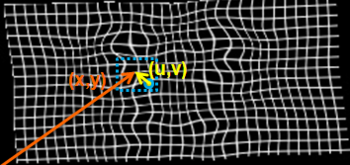
where [math]B_l[/math] is [math]l[/math]'th cubic B-spline basis function. [math](u,v,w)[/math] is the distance to [math](x,y,z)[/math] from the control point [math]\Phi_{i,j,k}[/math] as shown in Figure 2.
The deformation of a given point can be found using only the control points in the neighborhood of the given point. Therefore, optimization of the objective function can be implemented efficiently.
Implementation
We provide an efficient optimization scheme by using line search with the gradient descent algorithm. For computational efficiency, we employ a stochastic subsampling procedure. In each iteration of the algorithm, a random subset is drawn from all samples and the objective function is evaluated only on this sample set. The number of samples to be used in this method depends on the number of the parameters of the deformation field. Using the number of samples on the order of the number of variables works well in practice.
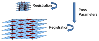
To obtain a dense deformation field capturing anatomical variations at different scales, we gradually increase the complexity of the deformation field by refining the grid of B-spline control points. First, we perform a global registration with affine transforms. Then, we use affine transforms to initialize a low resolution deformation field at a grid spacing around 32 voxels. We increase the resolution of the deformation field to 8 voxels by using registration results at coarser grids to initialize finer grids.

As in every iterative search algorithm, local minima pose a significant problem. To avoid local minima we use a multi-resolution optimization scheme for each resolution level of the deformation field. The registration is first performed at a coarse scale by downsampling the input. Results from coarser scales are used to initialize optimization at finer scales. For each resolution level of the deformation field we used a multi-resolution scheme of three image resolution levels.
We implemented our groupwise registration method in a multi-threaded fashion using Insight Toolkit (ITK) and made the implementation publicly available. We run experiments using a dataset of 50 MR images with $256\times256\times128$ voxels on a workstation with four CPUs and 8GB of memory. The running time of the algorithm is about 20 minutes for affine registration and two days for non-rigid registration of the entire dataset. The memory requirement of the algorithm depends linearly on the number of input images and was around 3GB for our dataset.
Progress
We tested the groupwise registration algorithm on a MR brain dataset and
compared the results to a pairwise approach \cite{joshi}.
The dataset consists of 50 MR brain images of three subgroups:
schizophrenics, affected disorder and normal control patients.
MR images are T1 scans with $256\times256\times128$ voxels
and $0.9375\times0.9375\times1.5$~$\mbox{mm}^3$ spacing.
MR images are preprocessed by skull stripping.
To account for global intensity variations, images are normalized
to have zero mean and unit variance.
For each image in the dataset, an automatic tissue classification \cite{pohl}
was performed, yielding gray matter (GM), white matter (WM) and cerebro-spinal
fluid (CSF) labels. In addition, manual segmentations of four subcortical regions
(left and right hippocampus and amygdala) and four cortical regions (left and right superior temporal
gyrus and para-hippocampus) were available for each MR image.
The prediction accuracy reported in Table \ref{table:pred} is lower than what is typically
achieved by segmentation methods. This is to be expected as our
relatively simple label prediction method only considers voxelwise
majority of the labels in the population and does not use the novel
image intensity to predict the labels. Effectively, Table \ref{table:pred} reports
the accuracy of the spatial prior (atlas) in predicting the labels
before the local intensity is used to refine the segmentation.
Increasing the complexity of the deformation model improves the
accuracy of prediction. An interesting open problem is automatically
identifying the appropriate deformation complexity before the
registration overfits and the accuracy of prediction goes down. We
also note that the alignment of the subcortical structures is much
better than that of the cortical regions. It is not surprising as the
registration algorithm does not use the information about geometry of the cortex
to optimize the alignment of the cortex. In addition, it has
been often observed that the cortical structures exhibit higher
variability across subjects when considered in the 3D volume rather
than modelled on the surface.
Our experiments highlight the need for further research in developing evaluation criteria for image alignment. We used the standard Dice measure, but it is not clear that this measurement captures all the nuances of the resulting alignment.
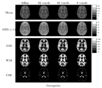
Comparing the groupwise registration to the pairwise approach, we observe that the sharpness of the mean images and the tissue overlaps in Figure~\ref{fig:mean} look visually similar. From Table~\ref{table:pred}, we note that groupwise registration performs slightly better than the pairwise setting in most of the cases, especially as we increase the complexity of the warp. This suggests that considering the population as a whole and registering subjects jointly brings the population into better alignment than matching each subject to a mean template image. However, the advantage shown here is only slight; more comparative studies are needed of the two approaches.
%Average Dice measures in Table \ref{table:pred} indicate relatively low values, especially for %manual segmentations of cortical structures. %This is to be expected as our relatively simple label prediction method %only considers voxelwise majority of the labels in the population. %Higher overlap values can be obtained by using more advanced segmentation techniques which make us of the % shapes of the structures. %As our method keeps the voxelwise intensity distributions in the population, these distributions %can be used to supply prior information to a more advanced segmentation algorithm to increase %the segmentation accuracy.
%Evaluation of a groupwise registration
%challenging task as it is hard to distinguish between registration inaccuracy and anatomical variability
%by considering Dice measure as the only evaluation criterion.
%However, comparing overlap measures relative to each other gives us useful information.
%The blurriness of the mean images in figure \ref{fig:mean} indicate high anatomical variabilities
%at cortical structures.
%Part of this anatomical variability is captured by higher resolution levels of B-splines,
%as can be observed from the increase in Dice measures for cortical structures in Table \ref{table:pred}.
%White matter and grey matter tissue type have a significant component in cortical regions; therefore,
%the overlap measures for these tissue types also increase as the resolution of the deformation field increases.
%Label overlap values for subcortical structures do not improve significantly with an increase in the resolution of the
%deformation field.
%These structures do not highly correlate with local intensity variations; therefore,
%we believe that
%the low Dice measures are mostly due to anatomical variabilities in these structures.
%As for the comparison of groupwise to pairwise approach, %we can observe that the sharpness of the mean images and the tissue overlaps in figure \ref{fig:mean} look visually similar. %From figure \ref{table:pred} we note that groupwise registration performs %slightly better than the pairwise setting in most of the cases. %This suggests that considering the population as a whole and registering subjects jointly brings the population into better %alignment than matching each subject to a mean template image. %A mean template image cannot fully explain multi-modal distributions; our groupwise setting %captures the modes in the distributions by considering stack entropies as an alignment criterion.
We compare our groupwise algorithm to a pairwise method where we register each subject to the mean intensity using sum of square differences. The objective function for pairwise registration to the mean can be described as follows [math] f_{pair} = \sum_{n=1}^{N} ( I_n(T_n(x)) - \mu(x) )^2 [/math] where $\mu$ is defined as the mean of the intensities $\mu(x) = \frac{1}{N}\sum_{n=1}^{N} I_n(T_n(x))$. During each iteration we consider the mean image as a reference image and register every subject to the mean image using sum of squared differences. After each iteration the mean image is updated and pairwise registrations are performed until convergence.
The images in Figure \ref{fig:mean} show central slices of 3D images after registration. Visually, mean images get sharper and variance images becomes darker, especially around central ventricles and cortical regions. We can observe that anatomical variability at cortical regions causes significant blur for GM, WM and CSF structures using affine registration. Finer scales of B-spline deformation fields capture a significant part of this anatomical variability and the tissue label overlap images get sharper.
We evaluate registration results by measuring label prediction accuracy in a leave-one-out fashion for the two different sets of segmentation labels. To predict the segmentation labels of a subject, we use majority voting for the labels in the rest of the population. We compute the Dice measure between the predicted and the true labels and average
over the whole population.
%Table \ref{table:pred} shows average Dice measures for two automatically segmented %tissue types: grey matter (GM) and white matter (WM) in the first two columns. %We excluded cerebro-spinal fluid (CSF) from the evaluation because CSF labels %near the cortex get corrupted %after preprocessing the data with skull stripping. %In the last two columns of Table \ref{table:pred} we display average prediction values for %manual segmentations of the cortical structures: superior temporal gyrus and para-hippocampus in the %left and right hemispheres; the subcortical structures: amygdala and hippocampus in the left and %right hemispheres.
Key Investigators
- S.K. Balci, P. Golland, S. Wells, M.R. Sabuncu, S. Bouix, M. Shenton.
Publications
- S.K. Balci, P. Golland, M.E. Shenton, W.M. Wells III. Free-Form B-spline Deformation Model for Groupwise Registration. In Proceedings of MICCAI 2007 Statistical Registration Workshop: Pair-wise and Group-wise Alignment and Atlas Formation, 23-30, 2007.


