Difference between revisions of "Projects:LongitudinalShapeAnalysis"
Jfishbaugh (talk | contribs) |
Jfishbaugh (talk | contribs) |
||
| Line 30: | Line 30: | ||
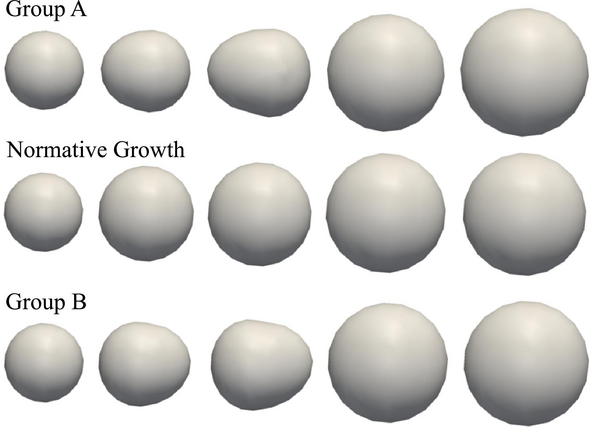
'''Synthetic Data''' We first evaluate our framework with a database of synthetic longitudinal shape data. In this simple database, normative growth is modeled by a sphere which grows isotropically over time. We further consider two groups, A and B, with different patterns of growth. Group A starts as a small sphere, develops a protuberance in the negative x direction, and eventually evolves into large sphere. Group B also starts from a small sphere, but develops a protuberance in the positive x direction, before evolving into a large sphere. Subjects from both groups contain 5 time points corresponding to 6, 10, 12, 18, and 24 months. We construct 12 subjects in each group by randomizing the amount of protuberance and also the amount of global scaling. A typical subject from group A and group B as well as the normative reference growth are summarized in Fig 2. | '''Synthetic Data''' We first evaluate our framework with a database of synthetic longitudinal shape data. In this simple database, normative growth is modeled by a sphere which grows isotropically over time. We further consider two groups, A and B, with different patterns of growth. Group A starts as a small sphere, develops a protuberance in the negative x direction, and eventually evolves into large sphere. Group B also starts from a small sphere, but develops a protuberance in the positive x direction, before evolving into a large sphere. Subjects from both groups contain 5 time points corresponding to 6, 10, 12, 18, and 24 months. We construct 12 subjects in each group by randomizing the amount of protuberance and also the amount of global scaling. A typical subject from group A and group B as well as the normative reference growth are summarized in Fig 2. | ||
| + | |||
| + | [[File:Synth_example_database_medium.png|600px|center|thumb|'''Fig. 2.''' Fig. 2. The synthetic shape database with observations at 6, 10, 12, 18, and 24 months. '''Top:''' Typical shape observations for a subject from group A. Middle: The normative growth scenario. '''Bottom:''' Typical shape observations for a subject from group B.]] | ||
= Literature = | = Literature = | ||
Revision as of 17:58, 15 August 2012
Home < Projects:LongitudinalShapeAnalysisBack to Utah 2 Algorithms
Ongoing Work (Updated 8/14/12)
Analysis of Longitudinal Shape Variability
Quantification of anatomical variability within a population and between populations are fundamental tasks in medical imaging studies. In many clinical applications, it is particularly crucial to quantify anatomical variability over time in order to determine disease progression and to isolate clinically important differences in both space and time. Such studies are designed around longitudinal imaging, where we acquire repeated measurements over time of the same subject, which yields rich data for analysis. Statistical analysis of longitudinal anatomical data is a problem with significant challenges due to the difficulty in modeling anatomical changes, such as growth, and comparing changes across different populations.
In this project, we propose a new approach for analyzing statistical variability of shapes over time, in the spirit of which is based on combining cross-sectional atlas construction with subject specific growth modeling. The growth model used for shape regression naturally handles multiple shapes at each time point and does not require point correspondence between subjects, making the proposed framework both convenient and applicable to a wide range of clinical problems.
Description
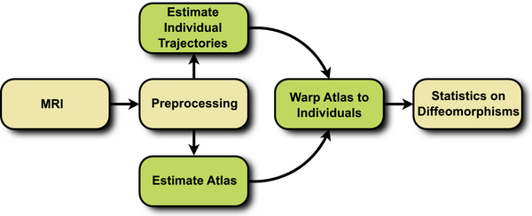
The proposed framework consists of three steps, summarized in Fig. 1. First, a cross-sectional atlas is estimated by shape regression, which can be thought of Fig. 1. Flowchart depicting the proposed method. as normative, reference evolution. Second, subject specific growth trajectories are estimated independently for each individual, accounting for intra-subject variability. Third, a homologous space for statistical analysis is obtained by warping the atlas to each individual at any time point of interest.
The first two steps require the estimation of a growth model, the specifics of which are discussed in the next section. Here we use the acceleration controlled growth model of [1], where shape evolution is modeled as a continuous flow of deformation. A baseline shape is continuously deformed over time to match the target shapes. The estimation is posed as a variational problem balancing fidelity to data with regularity.
The parameterization by acceleration guarantees that the estimated evolution is temporally smooth. Furthermore, the acceleration controlled growth model is generic, with no constraint that the flow of deformation must follow a geodesic path, or close to a geodesic path. For measuring shape similarity, we use the metric on currents [2]. This way, shapes are modeled as distributions, alleviating the need for explicit point correspondence between shapes.
We extract shape features, which are diffeomorphisms that map the reference atlas to each subject at a specific time point. This is accomplished by warping the atlas to each subject at the time point of interest using the registration framework of [10]. Due to regression, we can construct a shape from the atlas and from any individual at any time of interest. The warping from atlas space to each individual establishes homologous points between every subject.
The flow of diffeomorphisms that warp the template shape to each individual subject shape are geodesic [3]. As a result, the initial momenta completely determine the entire deformation. Since the atlas is warped to each subject, every diffeomorphism starts from the same reference space. We can leverage this common vector space to compute intrinsic statistics. For example, a mean can be computed by simply taking the arithmetic mean of a collection of momenta fields. The mean momenta can then be applied to a shape via geodesic shooting.
Results
Synthetic Data We first evaluate our framework with a database of synthetic longitudinal shape data. In this simple database, normative growth is modeled by a sphere which grows isotropically over time. We further consider two groups, A and B, with different patterns of growth. Group A starts as a small sphere, develops a protuberance in the negative x direction, and eventually evolves into large sphere. Group B also starts from a small sphere, but develops a protuberance in the positive x direction, before evolving into a large sphere. Subjects from both groups contain 5 time points corresponding to 6, 10, 12, 18, and 24 months. We construct 12 subjects in each group by randomizing the amount of protuberance and also the amount of global scaling. A typical subject from group A and group B as well as the normative reference growth are summarized in Fig 2.
Literature
[1] Fishbaugh, J., Durrleman, S., Gerig, G.: Estimation of smooth growth trajectories with controlled acceleration from time series shape data. In: Fichtinger, G., Peters, T. (eds.) MICCAI. LNCS, vol. 6892, pp. 401–408. Springer (2011)
[2] Vaillant, M., Glaun`es, J.: Surface matching via currents. In: IPMI. LNCS, vol. 3565, pp. 381–392. Springer (2005)
[3] Miller, M, I., Trouv´e, A., Younes, L.: On the metrics and Euler-Lagrange equations of Computational Anatomy. Annual Review of Biomedical Engineering 4, 375–405 (2002)
Key Investigators
- Utah: James Fishbaugh, Marcel Prastawa, Guido Gerig
- INRIA/ICM, Pitie Salpetriere Hospital: Stanley Durrleman
- Carolina Institute for Developmental Disabilities: Joseph Piven

