Difference between revisions of "Slicer3:Python"
| Line 92: | Line 92: | ||
[[Image:PythonAfter.png]] | [[Image:PythonAfter.png]] | ||
| + | |||
| + | ==== MatPlotLib tutorial ==== | ||
| + | The [http://matplotlib.sourceforge.net/ MatPlotLib] interface should be familiar to Matlab users, as the design philosophy is the same (indeed, MatPlotLib is nearly identical, but free!). This tutorial assumes you have installed [http://sourceforge.net/projects/matplotlib MatPlotLib] and have followed the tutorials above. | ||
| + | |||
| + | >>> # import MatPlotLib via pylab functions so we can refer to them directly | ||
| + | >>> from pylab import * | ||
| + | >>> imshow ( data[128,:,:] ) | ||
| + | >>> # Instruct pylab to show our plots... hit return to continue entering commands. | ||
| + | >>> show() | ||
| + | |||
| + | [[Image:Pythonimshow.png]] | ||
| + | |||
| + | >>> # Clear the plot | ||
| + | >>> clf() | ||
| + | >>> # Be warned: hist takes some time on an image | ||
| + | >>> hist ( data, 20 ) | ||
| + | (array([10813255, 1065860, 1106656, 802983, 761897, 730788, | ||
| + | 637444, 470011, 297534, 152217, 82640, 43318, | ||
| + | 26781, 16333, 11464, 8095, 6386, 4084, | ||
| + | 1419, 195]), array([ 0. , 31.5, 63. , 94.5, 126. , 157.5, 189. , 220.5, | ||
| + | 252. , 283.5, 315. , 346.5, 378. , 409.5, 441. , 472.5, | ||
| + | 504. , 535.5, 567. , 598.5]), <a list of 20 Patch objects>) | ||
| + | |||
| + | [[Image:Pythonhist.png]] | ||
Revision as of 16:15, 12 February 2007
Home < Slicer3:PythonContents
Python for scientific computing
Python has a fairly comprehensive package for scientific computing called SciPy. Of main interest to Slicer users/developers is NumPy. NumPy provides most of the features of the Matlab image processing toolbox and numeric computations, but in an Open Source package. A compelling reason to use NumPy is the ease of interaction and integration with Slicer3.
Slicer3 and Python
At the recent Slicer3 Mini-Retreat, a Python interpreter was added to the Slicer build. This may be built by following these steps.
- Install Python 2.4 or later
- Install NumPy, be sure to find the correct installer for your version of Python
- Optional: Install SciPy which is used in the tutorials below
- Optional: Install MatPlotLib, a NumPy plotting package developed to emulate Matlab's plotting capabilities. Used in the tutorials.
- Run CMake setting the "USE_PYTHON" option, and setting the path to your Python installation
- Check Advanced Options
- Verify that CMake found your Python installation
- Compile Slicer
- It is best to clean the SlicerBaseGUI project, as this may not be correctly rebuilt.
- A new build target SlicerGUIPython should appear
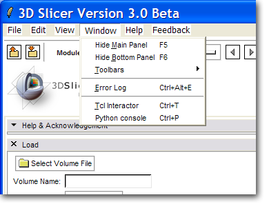
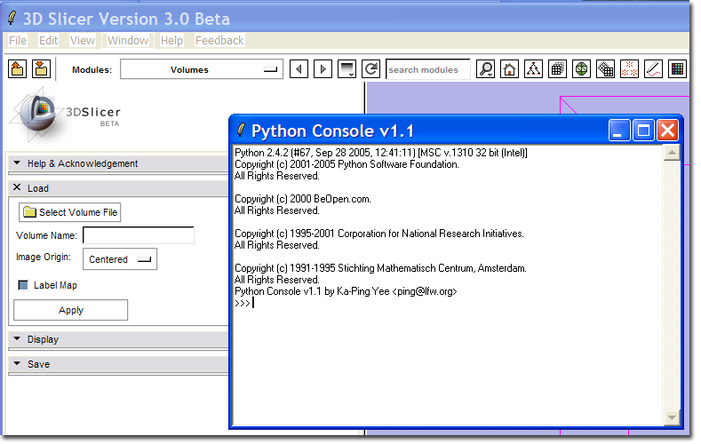
A new menu command Python Interpreter should appear on the Window menu.
This command should bring up the Python Console window.
Basic Slicer/Python tutorial
Note: this is initial documentation only, and is subject to change as the API evolves.
The Slicer Python interpreter has access to all Python modules referenced by the environment variable PYTHONPATH as well as the Slicer internal module. The Slicer module also supports the interface between Slicer Volume Nodes and NumPy. It would be instructive for the reader to review the NumPy documentation. For serious users of NumPy, there is the Guide to NumPy by Travis Oliphant for purchase.
In this example, a volume named T2_MGH.nhdr has been loaded into Slicer.
Listing available datasets
>>> import Slicer
>>> help ( Slicer.ListVolumeNodes )
Help on function ListVolumeNodes in module Slicer:

ListVolumeNodes()
    Returns a dictionary containing the index and
    vtkMRMLVolumeNodes currently loaded by Slicer

>>> nodes = Slicer.ListVolumeNodes()
>>> nodes
{0: vtkTemp1554}
>>> t2 = nodes[0]
>>> t2.GetName()
'T2_MGH.nhdr'
>>> t2.GetSpacing()
'0.84375 0.84375 0.84 '
>>> print t2.ListMethods()
<<<Output truncated>>>
Help on most Python functions is available using the built in help() command. This example shows how to list the available MRML volumes loaded by Slicer, select the volume you would like to use, and print some information from the volume. An exhaustive list of methods defined on each volume can be found using the ListMethods() method on the volume node.
NumPy tutorial
Python and NumPy give direct access to the volume data in Slicer by wrapping the image data in a NumPy array object through the .ToArray() method on the volume node. This tutorial assumes you have installed SciPy.
>>> # Access the image data directly
>>> data = t2.GetImageData().ToArray()
>>> print data
[[[ 0  0  0 ...,  0  0  0]
  [ 0  0  1 ...,  0  1  0]
  [ 0  0  0 ...,  0  0  0]
  ...,
  [ 0  8  0 ...,  0  1  2]
  [ 0  0  0 ...,  4  1  2]
  [ 0  0  2 ...,  6  0  2]]

<<< Some output truncated >>>

 [[ 0  0  0 ...,  0  0  0]
  [ 0  0  0 ...,  0  0  0]
  [ 0  0  0 ...,  0  0  0]
  ...,
  [ 0  3  3 ...,  0  0  8]
  [ 0  6  0 ...,  5  3 13]
  [ 0  5  1 ...,  9  3  8]]]
>>> # Load the image filtering package from scipy
>>> import scipy.ndimage
>>> # Filter into a new array
>>> temp = scipy.ndimage.gaussian_filter ( data, 2.0 )
>>> # Copy back into Slicer
>>> data[:] = temp[:]
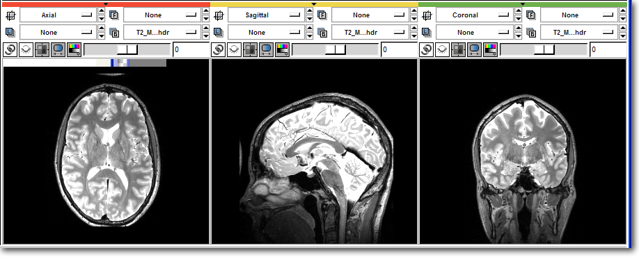
Before:
After:
MatPlotLib tutorial
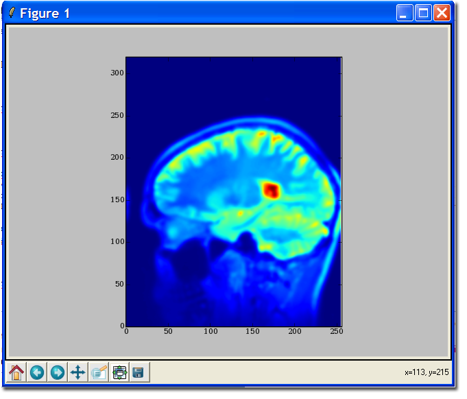
The MatPlotLib interface should be familiar to Matlab users, as the design philosophy is the same (indeed, MatPlotLib is nearly identical, but free!). This tutorial assumes you have installed MatPlotLib and have followed the tutorials above.
>>> # import MatPlotLib via pylab functions so we can refer to them directly
>>> from pylab import *
>>> imshow ( data[128,:,:] )
>>> # Instruct pylab to show our plots... hit return to continue entering commands.
>>> show()
>>> # Clear the plot
>>> clf()
>>> # Be warned: hist takes some time on an image
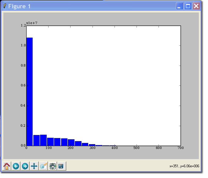
>>> hist ( data, 20 )
(array([10813255,  1065860,  1106656,   802983,   761897,   730788,
         637444,   470011,   297534,   152217,    82640,    43318,
          26781,    16333,    11464,     8095,     6386,     4084,
           1419,      195]), array([   0. ,   31.5,   63. ,   94.5,  126. ,  157.5,  189. ,  220.5,
        252. ,  283.5,  315. ,  346.5,  378. ,  409.5,  441. ,  472.5,
        504. ,  535.5,  567. ,  598.5]), <a list of 20 Patch objects>)
