Projects:BrainConnectivity

Back to NA-MIC Collaborations, MIT Algorithms

Our goal is to use measures of connectivity between various ROIs as an avenue for understanding the structural and functional organization of the brain. We assess functional and anatomical connectivity using both fMRI correlations and DWI tractography measures, respectively.

Joint Modeling of Anatomical and Functional Connectivity for Population Studies

The interaction between functional and anatomical connectivity provides a rich framework for understanding the brain. Functional connectivity is commonly measured via temporal correlations in resting-state fMRI data. These correlations are believed to reflect the intrinsic functional organization of the brain. Anatomical connectivity is often measured using DWI tractography, which estimates the configuration of underlying white matter fibers. In this work we propose and demonstrate a novel probabilistic framework to infer the relationship between these modalities. The model is based on latent connectivities between brain regions and makes intuitive assumptions about the data generation process. We present a natural extension of the model to population studies, which we use to identify widespread connectivity changes in schizophrenia.

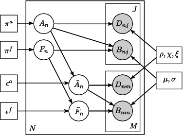
Fig 1. Joint model for the effects of schizophrenia. The pairwise connections are indexed with [math]n=1[/math].

Unlike voxel- and ROI-based analysis, we model the behavior of pairwise connections between regions of the brain. We define two latent variables: anatomical connectivity is a binary random variable that indicates the presence or absence of a direct anatomical pathway between the regions. Functional connectivity is a tri-state random variable that represent little or no functional co-activation, positive functional synchrony, and negative functional synchrony between the regions. Our observed variables are correlations in resting-state fMRI and average FA values along the white matter tracts. We model differences between the groups within the latent connectivities alone and share the data likelihood distributions between the two populations.

Experimental Results

We demonstrate our model on a study of 18 male patients with chronic schizophrenia and 18 male healthy controls. For each subject, an anatomical scan (SPGR, TR=7.4s, TE=3ms, FOV=26cm^2, res=1mm^3), a diffusion-weighted scan (EPI, TR=17s, TE=78ms, FOV=24cm^2, res=1.66x1.66x1.7mm, 51 gradient directions with b=900s/mm^2, 8 baseline scans with b=0s/mm^2) and a resting-state functional scan (EPI-BOLD, TR=3s, TE=30ms, FOV=24cm^2, res=1.875x1.875x3mm) were acquired using a 3T GE Echospeed system.

We segmented the structural images into 77 anatomical regions with Freesurfer. To inject prior clinical knowledge, we pre-selected 8 brain structures (corresponding to 16 regions) that are believed to play a role in schizophrenia: the superior temporal gyrus, rostral middle frontal gyrus, hippocampus, amygdala, posterior cingulate, rostral anterior cingulate, parahippocampal gyrus, and transverse temporal gyrus. We model only the 1096 unique pairwise connections between these ROIs and all other regions in the brain.

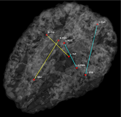
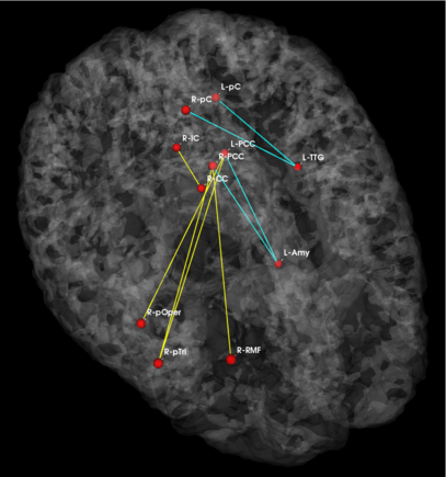
Fig 1. Significant anatomical and functional connectivity differences. Blue lines indicate higher connectivity in the control group; yellow lines indicate higher connectivity in the schizophrenia population.

Anatomical	Functional

Fig. 1 depicts the significantly different anatomical and functional connections identified by the algorithm. As seen, schizophrenia patients exhibit increased functional connectivity between the parietal/posterior cingulate region and the frontal lobe and reduced functional connectivity between the parietal/posterior cingulate region and the temporal lobe. These results confirm the hypotheses of widespread functional connectivity changes in schizophrenia and of functional abnormalities involving the default network.

The differences in anatomical connectivity implicate the superior temporal gyrus and hippocampus. We note that relatively few anatomical connections exhibit significant differences between the two populations. This may stem from our choice of ROIs. In particular, we rely on Freesurfer parcellations, which provide anatomically meaningful correspondences across subjects and mitigate the effects of minor registration errors. However, they may be too big to capture structural differences between the groups. We emphasize that our model can be easily applied to finer scale parcelations in future studies.

Table 1 reports classification accuracies for the generative model and SVM classifiers. Despite not being optimized for classification, our model exhibits above-chance generalization accuracy. We note that even the SVM does not achieve high discrimination accuracy. This underscores the well-documented challenge of finding robust functional and anatomical changes induced by schizophrenia. We stress that our main goal is to explain differences in connectivity. Classification is only presented for validation.

Table 1. Training and testing accuracy of ten-fold cross validation for the control (NC) and Schizophrenic (SZ) populations.

Robust Feature Selection in Functional Connectivity to Classify Schizophrenia Patients

Our motivation is to identify functional connectivity differences induced by schizophrenia. Schizophrenia is a disorder marked by widespread cognitive difficulties affecting intelligence, memory, and executive attention. These impairments are not localized to a particular cortical region; rather, they reflect abnormalities in widely-distributed functional and anatomical networks. Despite considerable interest in recent years, the origins and expression of the disease are still poorly understood.

Univariate tests and random effects analysis are, to a great extent, the standard in population studies of functional connectivity. Significantly different connections are identified using a score, which is computed independently for each functional correlation. Consequently, the analysis ignores important networks of connectivity within the brain. Moreover, due to the limited number of subjects, univariate tests are often done once using the entire dataset. Thus, stability of the method and of the results is rarely assessed.

In this paper we address the above limitations through ensemble learning. The Random Forest is an ensemble of decision tree classifiers that incorporates multiple levels of randomization. Each tree is grown using a random subset of the training data. Additionally, each node is constructed by searching over a random subset of features. The Random Forest derives a score for each feature, known as the Gini Importance (GI), which summarizes its discriminative power and can be used as an alternative to univariate statistics. This approach to feature selection confers several advantages. The randomization over subjects is designed to improve generalization accuracy, especially given a small number of training examples relative to the number of features. The randomization over features increases the likelihood of identifying all functional connections useful for group discrimination (rather than an uncorrelated subset). Finally, due to the ensemble-based learning, the Random Forest produces nonlinear decision boundaries. Hence, it can capture significant patterns of functional connectivity across distributed networks in the brain.

Experimental Results

We demonstrate our model on a study of 18 male patients with chronic schizophrenia and 18 male healthy controls. For each subject, an anatomical scan (SPGR, TR=7.4s, TE=3ms, FOV=26cm^2, res=1mm^3) and a resting-state functional scan (EPI-BOLD, TR=3s, TE=30ms, FOV=24cm^2, res=1.875x1.875x3mm) were acquired using a 3T GE Echospeed system.

The anatomical images were segmented into 77 regions using FreeSurfer. We performed standard functional connectivity pre-processing using both FSL and MATLAB. We extract fMRI connectivity between two anatomical regions by computing the Pearson correlation coefficient between every pair of voxels in these regions, applying a Fisher-r-to-z transform to each correlation (to enforce normality), and averaging these values. Since our regions are large, the correlation between the mean timecourses of the two regions shows poor correspondence with the distribution of voxel-wise correlations between them. Therefore, we believe our measure is more appropriate for assessing fMRI connectivity across subjects.

We use ten-fold cross-validation to quantify the performance of each method. The dataset is randomly divided into 10 subsets, each with an equal number of controls and schizophrenia patients. We then compute the Gini Importance values and t-scores using 9 of these subsets and reserve one for testing. During testing, we rank the functional correlations either by GI value or by t-score magnitude. Our assumption is that the significant differences between the control and clinical populations are contained in the first K features. We assess this hypothesis by training both a Random Forest classifier and a Radial Basis Function Support Vector Machine (RBF-SVM) using just these K functional correlations, and evaluating the classification accuracy on the held-out group. Utilizing multiple classifiers ensures a fair comparison between GI and univariate tests.

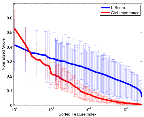
Fig 2. Stability of the GI values and t-scores on a log scale. For visualization, the values are normalized by the maximum GI and maximum t-score, respectively. Thick lines represent mean values, and the error bars correspond to standard deviations over the 100 cross-validation runs.

Fig. 2 depicts the stability of GI values and t-scores for each functional correlation across all 100 cross-validation runs. As seen, the t-scores exhibit far greater variability that the Gini Importance values. Additionally, the variance in GI is concentrated among the top features, whereas less-informative features are always assigned values near zero. Hence, although the top functional correlations may be ranked differently during each cross-validation run, the Random Forest isolates a consistent set of predictive features. In contrast, the t-scores vary uniformly over all features, regardless of significance. Thus, the set of predictive features can vary drastically over cross-validation runs.

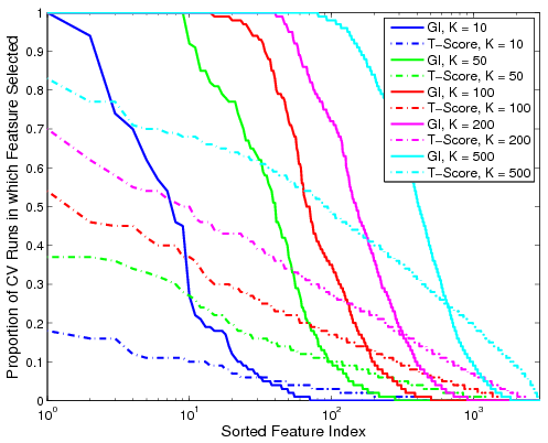
Fig 3. Proportion of the 100 cross-validation runs during which the feature is selected. The solid lines denote performance based on GI values for various K. The dashed lines represent the corresponding metric using t-scores.

Fig. 3 shows the proportion of cross-validation runs during which a particular functional correlation is ranked among the top K features, as measured by GI value or t-score. We observe that the decay in the proportion of iterations based on GI is relatively sharp from one to zero. Hence, if a feature is relevant for group discrimination, it tends to be ranked among the top; otherwise, it is almost always ignored. In contrast, feature selection based on t-scores is inconsistent and depends on the dataset. It is worth noting that none of the functional correlations are ranked in the top 500 by t-score for all 100 cross-validation iterations.

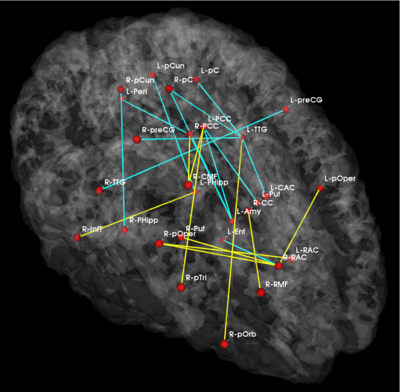
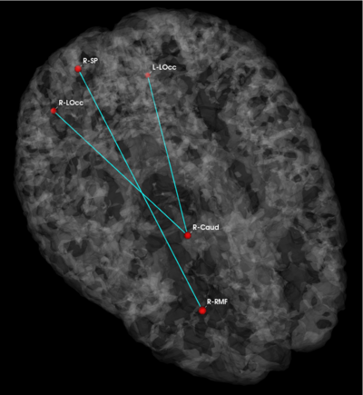
Fig 4. Connections selected during at least half of the cross-validation runs. Blue lines indicate higher connectivity in the control group; yellow lines indicate higher connectivity in the schizophrenia population.

Gini Importance	T-Score

Fig. 4 depicts the connections selected during at least half of the cross-validation iterations. Table XX reports the classification accuracy. For GI, we depict results for K=15, which yields the best classification accuracy. For t-score, we use K=150, which roughly corresponds to p-values less than 0.05. As seen, the significant functional correlations are disjoint between the feature selection methods. From these results, we conclude that the Gini Importance is a more robust feature selection criterion for clinical data than the univariate t-test.

Table 2. Training and testing accuracy of ten-fold cross validation using GI and t-score.

Exploration of Functional Connectivity via Clustering

Generative Model for Functional Connectivity

In the classical functional connectivity analysis, networks of interest are defined based on correlation with the mean time course of a user-selected `seed' region. Further, the user has to also specify a subject-specific threshold at which correlation values are deemed significant. In this project, we simultaneously estimate the optimal representative time courses that summarize the fMRI data well and the partition of the volume into a set of disjoint regions that are best explained by these representative time courses. This approach to functional connectivity analysis offers two advantages. First, is removes the sensitivity of the analysis to the details of the seed selection. Second, it substantially simplifies group analysis by eliminating the need for the subject-specific threshold. Our experimental results indicate that the functional segmentation provides a robust, anatomically meaningful and consistent model for functional connectivity in fMRI.

We formulate the problem of characterizing connectivity as a partition of voxels into subsets that are well characterized by a certain number of representative hypotheses, or time courses, based on the similarity of their time courses to each hypothesis. We model the fMRI signal at each voxel as generated by a mixture of Gaussian distributions whose centers are the desired representative time courses. Using the EM algorithm to solve the corresponding model-fitting problem, we alternatively estimate the representative time courses and cluster assignments to improve our random initialization.

Experimental Results

We used data from 7 subjects with a diverse set of visual experiments including localizer, morphing, rest, internal tasks, and movie. The functional scans were pre-processed for motion artifacts, manually aligned into the Talairach coordinate system, detrended (removing linear trends in the baseline activation) and smoothed (8mm kernel).

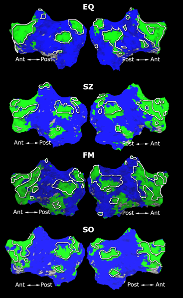
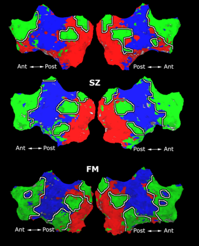
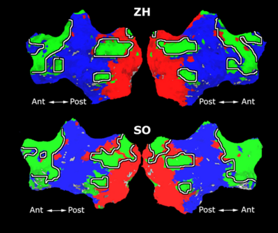
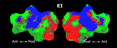
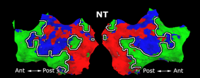
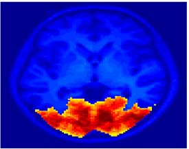
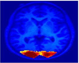
Fig. 5 shows the 2-system partition extracted in each subject independently of all others. It also displays the boundaries of the intrinsic system determined through the traditional seed selection, showing good agreement between the two partitions. Fig. 6 presents the results of further clustering the stimulus-driven cluster into two clusters independently for each subject.

Fig 5. 2-System Parcelation. Results for all 7 subjects.	Fig 6. 3-System Parcelation. Results for all 7 subjects.

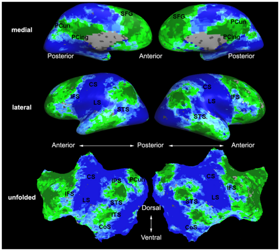
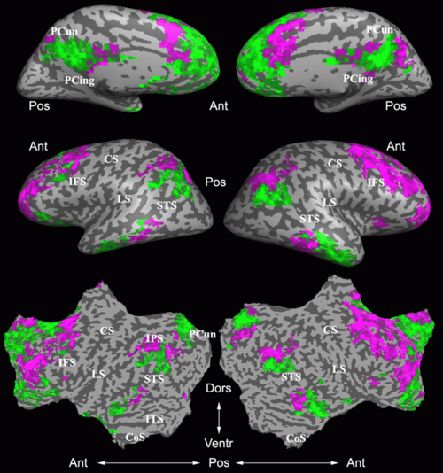
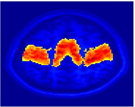
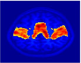
Fig. 7 presents the group average of the subject-specific 2-system maps. Color shading shows the proportion of subjects whose clustering agreed with the majority label. Fig. 8 shows the group average of a further parcelation of the intrinsic system, i.e., one of two clusters associated with the non-stimulus-driven regions. In order to present a validation of the method, we compare these results with the conventional scheme for detection of visually responsive areas. In Fig. 9, color shows the statistical parametric map while solid lines indicate the boundaries of the visual system obtained through clustering. The result illustrate the agreement between the two methods.

Fig 7. 2-System Parcellation. Group-wise result.	Fig 8. Validation: Parcelation of the intrinsic system.

Fig 9. Validation: Visual system.

Comparison between Different Clustering Schemes

As a continuation to the above experiments, we apply two distinct clustering algorithms to functional connectivity analysis: K-Means clustering and Spectral Clustering. The K-Means algorithm assumes that each voxel time course is drawn independently from one of k multivariate Gaussian distributions with unique means and spherical covariances. In contrast, Spectral Clustering does not presume any parametric form for the data. Rather it captures the underlying signal geometry by inducing a low-dimensional representation based on a pairwise affinity matrix constructed from the data. Without placing any a priori constraints, both clustering methods yield partitions that are associated with brain systems traditionally identified via seed-based correlation analysis. Our empirical results suggest that clustering provides a valuable tool for functional connectivity analysis.

One downside of Spectral Clustering is that it relies on the eigen-decomposition of an NxN affinity matrix, where N is the number of voxels in the whole brain. Since N is on the order of ~200,000 voxels, it is infeasible to compute the full eigen-decomposition given realistic memory and time constraints. To solve this problem, we approximate the leading eigenvalues and eigenvectors of the affinity matrix via the Nystrom Method. This is done by selecting a random subset of "Nystrom Samples" from the data. The affinity matrix and spectral decomposition is computed only for this subset, and the results are projected onto the remaining data points.

Experimental Results

We validate these algorithms on resting state data collected from 45 healthy young adults (mean age 21.5, 26 female). Four 2mm isotropic functional runs were acquired from each subject. Each scan lasted for 6m20s with TR = 5s. The first 4 time points in each run were discarded, yielding 72 time samples per run. The entire brain volume is partitioned into an increasing number of clusters. We perform standard preprocessing on each of the four runs, including motion correction by rigid body alignment of the volumes, slice timing correction and registration to the MNI atlas space. The data is spatially smoothed with a 6mm 3D Gaussian filter, temporally low-pass filtered using a 0.08Hz cutoff, and motion corrected via linear regression. Next, we estimate and remove contributions from the white matter, ventricle and whole brain regions (assuming a linear signal model). We mask the data to include only brain voxels and normalized the time courses to have zero mean and unit variance. Finally, we concatenate the four runs into a single time course for analysis.

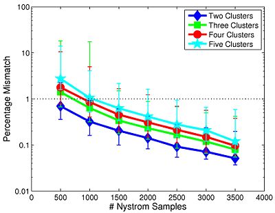
We first study the robustness of Spectral Clustering to the number of random samples. In this experiment, we start with a 4,000-sample Nystrom set, which is the computational limit of our machine. We then iteratively remove 500 samples and examine the effect on clustering performance. After matching the resulting clusters to those estimated with 4,000 samples, we compute the percentage of mismatched voxels between each trial and the 4,000-sample template. This procedure is repeated twice for each participant.

Fig 10. Varying the number of Nystrom Samples	Fig 11. Nystrom consistency for 2,000 random samples

Fig 10. depicts the median clustering difference when varying the number of Nystrom samples. Values represent the percentage of mismatched voxels w.r.t. the 4,000-sample template. Error bars delineate the 10th-90 percentile region. The median clustering difference is less than 1% for 1,000 or more Nystrom samples, and the 90th percentile difference is less than 1% for 1,500 or more samples. This experiment suggests that Nystrom-based SC converges to a stable clustering pattern as the number of samples increases. Based on these results, we chose to use 2,000 Nystrom samples for the remainder of this work. At this sample size, less than 5% of the runs for 2,4,5 clusters and approximately 8% of the runs for 3 clusters differed by more than 5% from the 4,000-sample template.

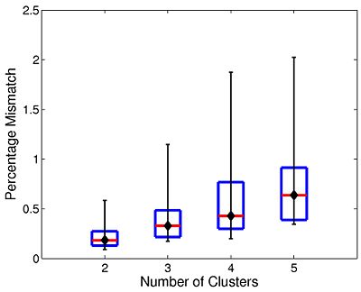
The box plot in Fig 11. summarizes the consistency of Nystrom-based Spectral Clustering across different random samplings. The red lines indicate median values, the box corresponds to the upper and lower quartiles, and error bars denote the 10th and 90th percentiles. Here, we perform SC 10 times on each participant using 2,000 Nystrom samples. We then align the cluster maps and compute the percentage of mismatched voxels between each unique pair of runs. This yields a total of 45 comparisons per participant. In all cases, the median clustering difference is less than 1%, and the 90th percentile value is less than 2.1%. Empirically, we find that Nystrom SC predictably converges to a second or third cluster pattern in only a handful of participants. This experiment suggests that we can obtain consistent clusterings with only 2,000 Nystrom samples.

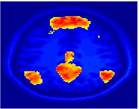
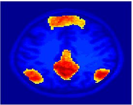
Fig 12. Clustering results across participants. The brain is partitioned into 5 clusters using Spectral Clustering/K-Means, and various seed are selected for Seed-Based Analysis. The color indicates the proportion of participants for whom the voxel was included in the detected system.

Spectral Clustering	K-Means	Seed-Based
Cluster 1, Slice 37	Cluster 1, Slice 37	PCC, Slice 37
Cluster 1, Slice 55	Cluster 1, Slice 55	vACC, Slice 55
Cluster 2, Slice 55	Cluster 2, Slice 55	Visual, Slice 55
Cluster 3, Slice 31	Cluster 3, Slice 31	Motor, Slice 31
Cluster 4, Slice 31	Cluster 4, Slice 31	IPS, Slice 31
Cluster 5, Slice 37	Cluster 5, Slice 37

Fig 12. shows clearly that both Spectral Clustering and K-Means can identify well-known structures such as the default network, the visual cortex, the motor cortex, and the dorsal attention system. Spectral Clustering and K-Means also identified white matter. In general, one would not attempt to delineate this region using seed-based correlation analysis because we regress out the white matter signal during the preprocessing. In our experiments Spectral Clustering and K-Means achieve similar clustering results across participants. Furthermore, both methods identify the same functional systems as seed-based analysis without requiring a priori knowledge about the brain and without significant computation. Thus, clustering algorithms offer a viable alternative to standard functional connectivity analysis techniques.

Comparison of ICA and Clustering for the Identification of Functional Connectivity in fMRI

Although ICA and clustering rely on very different assumptions on the underlying distributions, they produce surprisingly similar results for signals with large variation. Our main goal is to evaluate and compare the performance of ICA and clustering based on Gaussian mixture model (GMM) for identification of functional connectivity. Using the synthetic data with artificial activations and artifacts under various levels of length of the time course and signal-to-noise ratio of the data, we compare both spatial maps and their associated time courses estimated by ICA and GMM to each other and to the ground truth. We choose the number of sources via the model selection scheme, and compare all of the resulting components of GMM and ICA, not just the task-related components, after we match them component-wise using the Hungarian algorithm. This comparison scheme is verified in a high level visual cortex fMRI study. We find that ICA requires a smaller number of total components to extract the task-related components, but also needs a large number of total components to describe the entire data. We are currently applying ICA and clustering methods to connectivity analysis of schizophrenia patients.

Key Investigators

• MIT: Archana Venkataraman, Polina Golland
• Harvard: Carl-Frederik Westin, Marek Kubicki

Publications

NA-MIC Publications Database on Brain Connectivity