|
|
| (3 intermediate revisions by 3 users not shown) |
| Line 1: |
Line 1: |
| | Back to [[NA-MIC_Internal_Collaborations:fMRIAnalysis|NA-MIC Collaborations]], [[Algorithm:MIT|MIT Algorithms]] | | Back to [[NA-MIC_Internal_Collaborations:fMRIAnalysis|NA-MIC Collaborations]], [[Algorithm:MIT|MIT Algorithms]] |
| | __NOTOC__ | | __NOTOC__ |
| − | = fMRI Clustering = | + | = Improving fMRI Analysis using Supervised and Unsupervised Learning = |
| | | | |
| − | One of the major goals in analysis of fMRI data is the detection of networks in the brain with similar functional behavior. A wide variety of methods including hypothesis-driven statistical tests, unsupervised learning methods such as PCA and ICA, and different clustering algorithms have been employed to find these networks. This project aims to particularly study application of model-based clustering algorithms in identification of functional connectivity in the brain. | + | One of the major goals in the analysis of fMRI data is the detection of regions of the brain with similar functional behavior. A wide variety of methods including hypothesis-driven statistical tests, supervised, and unsupervised learning methods have been employed to find these networks. In this project, we develop novel learning algorithms that enable more efficient inferences from fMRI measurements. |
| | | | |
| − | = Clustering for the Exploration of Functional Connectivity = | + | = Clustering for Discovering Structure in the Space of Functional Selectivity = |
| | | | |
| − | '''''Generative Model for Functional Connectivity'''''
| + | We are devising clustering algorithms for discovering structure in the functional organization of the high-level visual cortex. It is suggested that there are regions in the visual cortex with high selectivity to certain categories of visual stimuli; we refer to these regions as /functional units/. Currently, the conventional method for detection of these regions is based on statistical tests comparing response of each voxel in the brain to different visual categories to see if it shows considerably higher activation to one category. For example, the well-known FFA (Fusiform Face Area) is the set of voxels which show high activation to face images. We use a model-based clustering approach to the analysis of this type of data as a means to make this analysis automatic and further discover new structures in the high-level visual cortex. |
| | | | |
| − | In the classical functional connectivity analysis, networks of interest are
| + | We formulate a model-based clustering algorithm that simultaneously |
| − | defined based on correlation with the mean time course of a user-selected
| + | finds a set of activation profiles and their spatial maps from fMRI time courses. We validate |
| − | `seed' region. Further, the user has to also specify a subject-specific threshold at which correlation
| + | our method on data from studies of category selectivity in the visual |
| − | values are deemed significant. In this project, we simultaneously estimate the optimal
| + | cortex, demonstrating good agreement with findings from prior |
| − | representative time courses that summarize the fMRI data well and
| + | hypothesis-driven methods. This hierarchical model enables functional group analysis |
| − | the partition of the volume into a set of disjoint regions that are best
| + | independent of spatial correspondence among subjects. We have also developed a co-clustering extension of this |
| − | explained by these representative time courses. This approach to functional connectivity analysis offers two
| + | algorithm which can simultaneously find a set of clusters of voxels and categories |
| − | advantages. First, is removes the sensitivity of the analysis to the details
| + | of stimuli in experiments with diverse sets of stimulus categories. Our model is nonparametric, learning the numbers of clusters in both domains as well as the cluster parameters. |
| − | of the seed selection. Second, it substantially simplifies group analysis | |
| − | by eliminating the need for the subject-specific threshold. Our experimental results indicate that
| |
| − | the functional segmentation provides a robust, anatomically meaningful | |
| − | and consistent model for functional connectivity in fMRI.
| |
| | | | |
| − | We formulate the problem of characterizing connectivity as a partition of voxels into subsets that are well characterized by a certain number of representative hypotheses, or time courses, based on the similarity of their time courses to each hypothesis. We model the fMRI signal at each voxel as generated by a mixture of Gaussian distributions whose centers are the desired representative time courses. Using the EM algorithm to solve the corresponding model-fitting problem, we alternatively estimate the representative time courses and cluster assignments to improve our random initialization.
| + | Fig. 1 shows the categories learned by our algorithm on a study with 8 subjects. We split trials of each image into two groups of equal size and consider |
| | + | each group as an independent stimulus forming a total of 138 |
| | + | stimuli. Hence, we can examine the consistency of our stimulus categorization with respect to identical trials. Stimulus pairs |
| | + | corresponding to the same image are generally assigned to the same |
| | + | category, confirming the consistency of the resuls across |
| | + | trials. Category 1 corresponds to the scene images and, interestingly, also includes all images of |
| | + | trees. This may suggest a high level category structure that is not |
| | + | merely driven by low level features. Such a structure is even more |
| | + | evident in the 4th category where images of a tiger that has a large |
| | + | face join human faces. Some other animals are clustered together with human bodies in categories 2 and |
| | + | 9. Shoes and cars, which have similar shapes, are clustered together |
| | + | in category 3 while tools are mainly found in category 6. |
| | | | |
| − | ''' ''Experimental Results'' '''
| |
| | | | |
| − | We used data from 7 subjects with a diverse set of visual experiments including localizer, morphing, rest, internal tasks, and movie. The functional scans were pre-processed for motion artifacts, manually aligned into the Talairach coordinate system, detrended (removing linear trends in the
| + | {| |
| − | baseline activation) and smoothed (8mm kernel).
| + | |+ '''Fig 1. Categories learned from 8 subjects''' |
| | + | |align="center"|[[Image:Category_singlefile1.png |thumb|800px]] |
| | + | |} |
| | | | |
| − | Fig. 1 shows the 2-system partition extracted in each subject independently | + | Fig. 2 shows the cluster centers, or activation profiles, for the first 13 of 25 clusters learned by our method. We see salient category structure in our profiles. For instance, system 1 shows lower responses to cars, shoes, and tools compared to other stimuli. Since the images representing these three categories in our experiment are generally smaller in terms of pixel size, this system appears selective to lower level features (note that the highest probability of activation among shoes corresponds to the largest shoe 3). System 3 and system 8 seem less responsive to faces compared to all other stimuli. |
| − | of all others. It also displays the boundaries of the intrinsic system determined
| |
| − | through the traditional seed selection, showing good agreement between the two
| |
| − | partitions. Fig. 2 presents the results of further clustering the stimulus-driven cluster into two clusters independently for each subject.
| |
| | | | |
| − | <table>
| + | {| |
| − | <tr> <th> '''Fig 1. 2-System Parcelation. Results for all 7 subjects.''' <th> '''Fig 2. 3-System Parcelation. Results for all 7 subjects.'''
| + | |+ '''Fig 2. System profiles of posterior probabilities of activation for each system to different stimuli. The bar heights correspond to the posterior probability of activation.''' |
| − | <tr> <td align="center">
| + | |align="center"|[[Image:Hdpprofs_all_1.png |thumb|800px]] |
| − | [[Image:mit_fmri_clustering_parcellation2_shb1_4.png |400px]]
| + | |} |
| − | [[Image:mit_fmri_clustering_parcellation2_shb5_6.png |400px]]
| |
| − | [[Image:mit_fmri_clustering_parcellation2_shb7.png |400px]]
| |
| − | <td align="center">
| |
| − | [[Image:mit_fmri_clustering_parcellation3_shb1_3.png |400px]]
| |
| − | [[Image:mit_fmri_clustering_parcellation3_shb4_5.png |400px]] | |
| − | [[Image:mit_fmri_clustering_parcellation3_shb6.png |400px]]
| |
| − | [[Image:mit_fmri_clustering_parcellation3_shb7.png |400px]]
| |
| − | </table>
| |
| | | | |
| − | Fig.3 presents the group average of the subject-specific 2-system maps. Color shading shows the proportion of subjects whose clustering agreed with the majority label. Fig. 4 shows the group average of a further parcelation of the intrinsic system, i.e., one of two clusters associated with the non-stimulus-driven regions. In order to present a validation of the method, we compare these results with the conventional scheme for detection of visually responsive areas. In Fig. 5, color shows the statistical parametric map while solid lines indicate the boundaries of the visual system obtained through clustering. The result illustrate the agreement between the two methods. | + | Fig. 3 shows the membership maps for the systems 2, 9, and 12, selective for bodies, faces, and scenes, respectively, which our model learns in a completely unsupervised fashion from the data. For comparison, Fig. 4 shows the significance maps found by applying the conventional confirmatory t-test to the data from the same subject. While significance maps appear to be generally larger than the extent of systems identified by our method, a close inspection reveals that system membership maps include the peak voxels for their corresponding contrasts. |
| | | | |
| − | <table>
| + | {| |
| − | <tr><th> '''Fig 3. 2-System Parcellation. Group-wise result.''' <th> '''Fig 4. Validation: Parcelation of the intrinsic system.'''
| + | |+ '''Fig 3. Membership probability maps corresponding to systems 22, 9, and 12, selective respectively for bodies (magenta), scenes (yellow), and faces (cyan) in one subject.''' |
| − | <tr> <td align="center">
| + | |align="center"|[[Image:Sys_2_9_12_subj1.png |thumb|800px]] |
| − | [[Image:mit_fmri_clustering_parcellation2_xsub.png |thumb|570px]] | + | |} |
| − | <td align="center">
| |
| − | [[Image:mit_fmri_clustering_intrinsicsystem.png |thumb|500px]]
| |
| − | </table>
| |
| | | | |
| | {| | | {| |
| − | |+ '''Fig 5. Validation: Visual system.''' | + | |+ '''Fig 4. Map representing significance values for three contrasts: bodies-objects (magenta), faces-objects (cyan), and scenes-objects (yellow) in the same subject. Lighter colors correspond to higher significance.''' |
| − | |valign="top"|[[Image:mit_fmri_clustering_validation.png |thumb|1150px]] | + | |align="center"|[[Image:Sys_2_9_12_subj1.png |thumb|800px]] |
| | |} | | |} |
| | | | |
| − | '''''Comparison between Different Clustering Schemes''''' | + | '''''Earlier work''''' |
| − | | |
| − | As a continuation to the above experiments, we apply two distinct clustering algorithms to functional connectivity analysis: K-Means clustering and Spectral Clustering. The K-Means algorithm assumes that each voxel time course is drawn independently from one of <em>k</em> multivariate Gaussian distributions with unique means and spherical covariances. In contrast, Spectral Clustering does not presume any parametric form for the data. Rather it captures the underlying signal geometry by inducing a low-dimensional representation based on a pairwise affinity matrix constructed from the data. Without placing any <em>a priori</em> constraints, both clustering methods yield partitions that are associated with brain systems traditionally identified via seed-based correlation analysis. Our empirical results suggest that clustering provides a valuable tool for functional connectivity analysis.
| |
| − | | |
| − | One downside of Spectral Clustering is that it relies on the eigen-decomposition of an <em>NxN</em> affinity matrix, where <em>N</em> is the number of voxels in the whole brain. Since <em>N</em> is on the order of ~200,000 voxels, it is infeasible to compute the full eigen-decomposition given realistic memory and time constraints. To solve this problem, we approximate the leading eigenvalues and eigenvectors of the affinity matrix via the Nystrom Method. This is done by selecting a random subset of "Nystrom Samples" from the data. The affinity matrix and spectral decomposition is computed only for this subset, and the results are projected onto the remaining data points.
| |
| − | | |
| − | '''''Experimental Results'''''
| |
| − | | |
| − | We validate these algorithms on resting state data collected from 45 healthy young adults (mean age 21.5, 26 female). Four 2mm isotropic functional runs were acquired from each subject. Each scan lasted for 6m20s with TR = 5s. The first 4 time points in each run were discarded, yielding 72 time samples per run. The entire brain volume is partitioned into an increasing number of clusters. We perform standard preprocessing on each of the four runs, including motion correction by rigid body alignment of the volumes, slice timing correction and registration to the MNI atlas space. The data is spatially smoothed with a 6mm 3D Gaussian filter, temporally low-pass filtered using a 0.08Hz cutoff, and motion corrected via linear regression. Next, we estimate and remove contributions from the white matter, ventricle and whole brain regions (assuming a linear signal model). We mask the data to include only brain voxels and normalized the time courses to have zero mean and unit variance. Finally, we concatenate the four runs into a single time course for analysis.
| |
| − | | |
| − | We first study the robustness of Spectral Clustering to the number of random samples. In this experiment, we start with a 4,000-sample Nystrom set, which is the computational limit of our machine. We then iteratively remove 500 samples and examine the effect on clustering performance. After matching the resulting clusters to those estimated with 4,000 samples, we compute the percentage of mismatched voxels between each trial and the 4,000-sample template. This procedure is repeated twice for each participant.
| |
| − | | |
| − | <table>
| |
| − | <tr> <th> '''Fig 6. Varying the number of Nystrom Samples''' <th> '''Fig 7. Nystrom consistency for 2,000 random samples'''
| |
| − | <tr>
| |
| − | <td align="center">
| |
| − | [[Image:mit_fmri_clustering_Samples_LogMedian2.jpeg |400px]]
| |
| − | <td align="center">
| |
| − | [[Image:mit_fmri_clustering_Consistency_Box.jpeg |400px]]
| |
| − | </table>
| |
| − | | |
| − | Fig 6. depicts the median clustering difference when varying the number of Nystrom samples. Values represent the percentage of mismatched voxels w.r.t. the 4,000-sample template. Error bars delineate the <em>10th</em>-<em>90</em> percentile region. The median clustering difference is less than 1% for 1,000 or more Nystrom samples, and the <em>90th</em> percentile difference is less than 1% for 1,500 or more samples. This experiment suggests that Nystrom-based SC converges to a stable clustering pattern as the number of samples increases. Based on these results, we chose to use 2,000 Nystrom samples for the remainder of this work. At this sample size, less than 5% of the runs for 2,4,5 clusters and approximately 8% of the runs for 3 clusters differed by more than 5% from the 4,000-sample template.
| |
| − | | |
| − | The box plot in Fig 7. summarizes the consistency of Nystrom-based Spectral Clustering across
| |
| − | different random samplings. The red lines indicate median values, the box corresponds to the upper and lower quartiles, and error bars denote the <em>10th</em> and <em>90th</em> percentiles. Here, we perform SC 10 times on each participant using 2,000 Nystrom samples. We then align the cluster maps and compute the percentage of mismatched voxels between each unique pair of runs. This yields a total of 45 comparisons per participant. In all cases, the median clustering difference is less than 1%, and the <em>90th</em> percentile value is less than 2.1%. Empirically, we find that Nystrom SC predictably converges to a second or third cluster pattern in only a handful of participants. This experiment suggests that we can obtain consistent clusterings with only 2,000 Nystrom samples.
| |
| − | | |
| − | <table>
| |
| − | <tr> ''' Fig 8. Clustering results across participants. The brain is partitioned into 5 clusters using Spectral Clustering/K-Means, and various seed are selected for Seed-Based Analysis. The color indicates the proportion of participants for whom the voxel was included in the detected system.'''
| |
| − | <tr> <th> '''Spectral Clustering''' <th> '''K-Means''' <th> '''Seed-Based'''
| |
| − | <tr>
| |
| − | <td align="center">
| |
| − | [[Image:mit_fmri_clustering_SC_5Clust_2.jpeg |275px]]
| |
| − | <td align="center">
| |
| − | [[Image:mit_fmri_clustering_KM_5Clust_1.jpeg |275px]]
| |
| − | <td align="center">
| |
| − | [[Image:mit_fmri_clustering_Seed_PCC.jpeg |275px]]
| |
| − | <tr> <th> '''Cluster 1, Slice 37''' <th> '''Cluster 1, Slice 37''' <th> '''PCC, Slice 37'''
| |
| − | <tr>
| |
| − | <td align="center">
| |
| − | [[Image:mit_fmri_clustering_SC_5Double.jpeg |275px]]
| |
| − | <td align="center">
| |
| − | [[Image:mit_fmri_clustering_KM_5Double.jpeg |275px]]
| |
| − | <td align="center">
| |
| − | [[Image:mit_fmri_clustering_Seed_vACC.jpeg |275px]]
| |
| − | <tr> <th> '''Cluster 1, Slice 55''' <th> '''Cluster 1, Slice 55''' <th> '''vACC, Slice 55'''
| |
| − | <tr>
| |
| − | <td align="center">
| |
| − | [[Image:mit_fmri_clustering_SC_5Clust_3.jpeg |275px]]
| |
| − | <td align="center">
| |
| − | [[Image:mit_fmri_clustering_KM_5Clust_4.jpeg |275px]]
| |
| − | <td align="center">
| |
| − | [[Image:mit_fmri_clustering_Seed_V1.jpeg |275px]]
| |
| − | <tr> <th> '''Cluster 2, Slice 55''' <th> '''Cluster 2, Slice 55''' <th> '''Visual, Slice 55'''
| |
| − | <tr>
| |
| − | <td align="center">
| |
| − | [[Image:mit_fmri_clustering_SC_5Clust_4.jpeg |275px]]
| |
| − | <td align="center">
| |
| − | [[Image:mit_fmri_clustering_KM_5Clust_3.jpeg |275px]]
| |
| − | <td align="center">
| |
| − | [[Image:mit_fmri_clustering_Seed_M1.jpeg |275px]]
| |
| − | <tr> <th> '''Cluster 3, Slice 31''' <th> '''Cluster 3, Slice 31''' <th> '''Motor, Slice 31'''
| |
| − | <tr>
| |
| − | <td align="center">
| |
| − | [[Image:mit_fmri_clustering_SC_5Clust_1.jpeg |275px]]
| |
| − | <td align="center">
| |
| − | [[Image:mit_fmri_clustering_KM_5Clust_2.jpeg |275px]]
| |
| − | <td align="center">
| |
| − | [[Image:mit_fmri_clustering_Seed_IPS.jpeg |275px]]
| |
| − | <tr> <th> '''Cluster 4, Slice 31''' <th> '''Cluster 4, Slice 31''' <th> '''IPS, Slice 31'''
| |
| − | <tr>
| |
| − | <td align="center">
| |
| − | [[Image:mit_fmri_clustering_SC_5Clust_5.jpeg |275px]]
| |
| − | <td align="center">
| |
| − | [[Image:mit_fmri_clustering_KM_5Clust_5.jpeg |275px]]
| |
| − | <td align="center">
| |
| − | [[Image:mit_fmri_clustering_Colorbar2.jpeg |64px]]
| |
| − | <tr> <th> '''Cluster 5, Slice 37''' <th> '''Cluster 5, Slice 37''' <th>
| |
| − | </table>
| |
| − | | |
| − | Fig 8. shows clearly that both Spectral Clustering and K-Means can identify well-known structures such as the default network, the visual cortex, the motor cortex, and the dorsal attention system. Spectral Clustering and K-Means also identified white matter. In general, one would not attempt to delineate this region using seed-based correlation analysis because we regress out the white matter signal during the preprocessing. In our experiments Spectral Clustering and K-Means achieve similar clustering results across participants. Furthermore, both methods identify the same functional systems as seed-based analysis without requiring <em>a priori</em> knowledge about the brain and without significant computation. Thus, clustering algorithms offer a viable alternative to standard functional connectivity analysis techniques.
| |
| − | | |
| − |
| |
| − | ''' ''Comparison of ICA and Clustering for the Identification of Functional Connectivity in fMRI'' '''
| |
| − | | |
| − | Although ICA and clustering rely on very different assumptions on the underlying distributions, they produce surprisingly similar results for signals with large variation. Our main goal is to evaluate and compare the performance of ICA and clustering based on Gaussian mixture model (GMM) for identification of functional connectivity. Using the synthetic data with artificial activations and artifacts under various levels of length of the time course and signal-to-noise ratio of the data, we compare both spatial maps and their associated time courses estimated by ICA and GMM to each other and to the ground truth. We choose the number of sources via the model selection scheme, and compare all of the resulting components of GMM and ICA, not just the task-related components, after we match them component-wise using the Hungarian algorithm. This comparison scheme is verified in a high level visual cortex fMRI study. We find that ICA requires a smaller number of total components to extract the task-related components, but also needs a large number of total components to describe the entire data. We are currently applying ICA and clustering methods to connectivity analysis of schizophrenia patients.
| |
| − | | |
| − | = Clustering for Discovering Structure in the Space of Functional Selectivity =
| |
| − | | |
| − | ''' ''Clustering Study of Domain Specificity in High Level Visual Cortex'' '''
| |
| − | | |
| − | As a more specific application of model-based clustering algorithms, we are devising clustering algorithms for discovering structure in the functional organization of the high-level visual cortex. It is suggested that there are regions in the visual cortex with high selectivity to certain categories of visual stimuli. Currently, the conventional method for detection of these methods is based on statistical tests comparing response of each voxel in the brain to different visual categories to see if it shows considerably higher activation to one category. For example, the well-known FFA (Fusiform Face Area) is the set of voxels which show high activation to face images. We use a model-based clustering approach to the analysis of this type of data as a means to make this analysis automatic and further discover new structures in the high-level visual cortex.
| |
| − | | |
| − | Introducing the notion of space of activation
| |
| − | profiles, we construct a representation of the data which explicitly
| |
| − | parametrizes all interesting patterns of activation. Mapping the data into
| |
| − | this space, we formulate a model-based clustering algorithm that simultaneously
| |
| − | finds a set of activation profiles and their spatial maps. We validate
| |
| − | our method on the data from studies of category selectivity in visual
| |
| − | cortex, demonstrating good agreement with the findings based on prior
| |
| − | hypothesis-driven methods. This model enables functional group analysis
| |
| − | independent of spatial correspondence among subjects. We are currently working on a co-clustering extension of this
| |
| − | algorithm which can simultaneously find a set of clusters of voxels and meta-categories
| |
| − | of stimuli in experiments with diverse sets of stimulus categories.
| |
| | | | |
| − | Fig. 9 compares the map of voxels assigned to a face-selective profile by our algorithm with the t-test's map of voxels with statistically significant (p<0.0001) response to faces when compared with object stimuli. Note that in contrast with the hypothesis testing method, we don't specify the existence of a face-selective region in our algorithm and the algorithm automatically discovers such a profile of activation in the data. | + | Fig. 5 compares the map of voxels assigned to a face-selective profile by an earlier version of our algorithm with the t-test's map of voxels with statistically significant (p<0.0001) response to faces when compared with object stimuli. Note that in contrast with the hypothesis testing method, we don't specify the existence of a face-selective region in our algorithm and the algorithm automatically discovers such a profile of activation in the data. |
| | | | |
| | {| | | {| |
| − | |+ '''Fig 9. Spatial maps of the face selective regions found by the statistical test (red) and our mixture model (dark blue). Maps are presented in alternating rows for comparison. Visually responsive mask of voxels used in our experiment is illustrated in yellow and light blue.''' | + | |+ '''Fig 5. Spatial maps of the face selective regions found by the statistical test (red) and our mixture model (dark blue). Maps are presented in alternating rows for comparison. Visually responsive mask of voxels used in our experiment is illustrated in yellow and light blue.''' |
| | |align="center"|[[Image:mit_fmri_clustering_mapffacompare.PNG |thumb|800px]] | | |align="center"|[[Image:mit_fmri_clustering_mapffacompare.PNG |thumb|800px]] |
| | |} | | |} |
| Line 175: |
Line 67: |
| | '''''Hierarchical Model for Exploratory fMRI Analysis without Spatial Normalization''''' | | '''''Hierarchical Model for Exploratory fMRI Analysis without Spatial Normalization''''' |
| | | | |
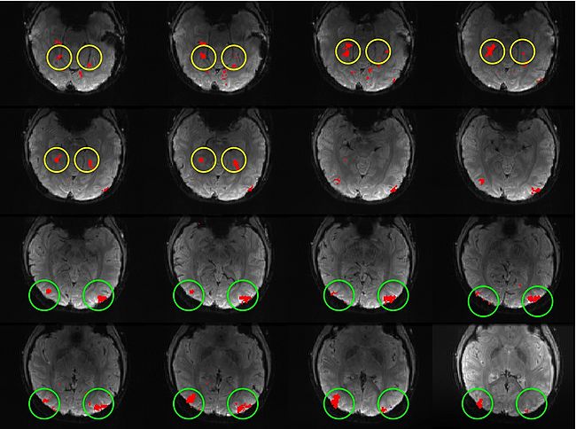
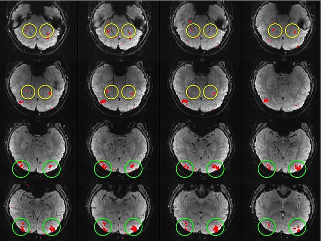
| − | Building on the work on the clustering model for the domain specificity, we develop a hierarchical exploratory method for simultaneous parcellation of multisub ect fMRI data into functionally coherent areas. The method is based on a solely functional representation of the fMRI data and a hierarchical probabilistic model that accounts for both inter-subject and intra-subject forms of variability in fMRI response. We employ a Variational Bayes approximation to fit the model to the data. The resulting algorithm finds a functional parcellation of the individual brains along with a set of population-level clusters, establishing correspondence between these two levels. The model eliminates the need for spatial normalization while still enabling us to fuse data from several subjects. We demonstrate the application of our method on the same visual fMRI study as before. Fig. 10 shows the scene-selective parcel in 2 different subjects. Parcel-level spatial correspondence is evident in the figure between the subjects. | + | Building on the work on the clustering model for the domain specificity, we develop a hierarchical exploratory method for simultaneous parcellation of multisub ect fMRI data into functionally coherent areas. The method is based on a solely functional representation of the fMRI data and a hierarchical probabilistic model that accounts for both inter-subject and intra-subject forms of variability in fMRI response. We employ a Variational Bayes approximation to fit the model to the data. The resulting algorithm finds a functional parcellation of the individual brains along with a set of population-level clusters, establishing correspondence between these two levels. The model eliminates the need for spatial normalization while still enabling us to fuse data from several subjects. We demonstrate the application of our method on the same visual fMRI study as before. Fig. 6 shows the scene-selective parcel in 2 different subjects. Parcel-level spatial correspondence is evident in the figure between the subjects. |
| | | | |
| | <table> | | <table> |
| − | <tr> <th> '''Fig 10. The map of the scene selective parcels in two different subjects. The rough location of the scene-selective areas PPA and TOS, identified by the expert, are shown on the maps by yellow and green circles, respectively.''' | + | <tr> <th> '''Fig 6. The map of the scene selective parcels in two different subjects. The rough location of the scene-selective areas PPA and TOS, identified by the expert, are shown on the maps by yellow and green circles, respectively.''' |
| | <tr> | | <tr> |
| | <td align="center"> | | <td align="center"> |
| Line 189: |
Line 81: |
| | = Key Investigators = | | = Key Investigators = |
| | | | |
| − | * MIT: Danial Lashkari, Archana Venkataraman, Ed Vul, Nancy Kanwisher, Polina Golland. | + | * MIT: Danial Lashkari, Archana Venkataraman, Ramesh Sridharan, Ed Vul, Nancy Kanwisher, Polina Golland. |
| | * Harvard: J. Oh, Marek Kubicki, Carl-Fredrik Westin. | | * Harvard: J. Oh, Marek Kubicki, Carl-Fredrik Westin. |
| | | | |
Back to NA-MIC Collaborations, MIT Algorithms
Improving fMRI Analysis using Supervised and Unsupervised Learning
One of the major goals in the analysis of fMRI data is the detection of regions of the brain with similar functional behavior. A wide variety of methods including hypothesis-driven statistical tests, supervised, and unsupervised learning methods have been employed to find these networks. In this project, we develop novel learning algorithms that enable more efficient inferences from fMRI measurements.
Clustering for Discovering Structure in the Space of Functional Selectivity
We are devising clustering algorithms for discovering structure in the functional organization of the high-level visual cortex. It is suggested that there are regions in the visual cortex with high selectivity to certain categories of visual stimuli; we refer to these regions as /functional units/. Currently, the conventional method for detection of these regions is based on statistical tests comparing response of each voxel in the brain to different visual categories to see if it shows considerably higher activation to one category. For example, the well-known FFA (Fusiform Face Area) is the set of voxels which show high activation to face images. We use a model-based clustering approach to the analysis of this type of data as a means to make this analysis automatic and further discover new structures in the high-level visual cortex.
We formulate a model-based clustering algorithm that simultaneously
finds a set of activation profiles and their spatial maps from fMRI time courses. We validate
our method on data from studies of category selectivity in the visual
cortex, demonstrating good agreement with findings from prior
hypothesis-driven methods. This hierarchical model enables functional group analysis
independent of spatial correspondence among subjects. We have also developed a co-clustering extension of this
algorithm which can simultaneously find a set of clusters of voxels and categories
of stimuli in experiments with diverse sets of stimulus categories. Our model is nonparametric, learning the numbers of clusters in both domains as well as the cluster parameters.
Fig. 1 shows the categories learned by our algorithm on a study with 8 subjects. We split trials of each image into two groups of equal size and consider
each group as an independent stimulus forming a total of 138
stimuli. Hence, we can examine the consistency of our stimulus categorization with respect to identical trials. Stimulus pairs
corresponding to the same image are generally assigned to the same
category, confirming the consistency of the resuls across
trials. Category 1 corresponds to the scene images and, interestingly, also includes all images of
trees. This may suggest a high level category structure that is not
merely driven by low level features. Such a structure is even more
evident in the 4th category where images of a tiger that has a large
face join human faces. Some other animals are clustered together with human bodies in categories 2 and
9. Shoes and cars, which have similar shapes, are clustered together
in category 3 while tools are mainly found in category 6.
Fig 1. Categories learned from 8 subjects
|
|
Fig. 2 shows the cluster centers, or activation profiles, for the first 13 of 25 clusters learned by our method. We see salient category structure in our profiles. For instance, system 1 shows lower responses to cars, shoes, and tools compared to other stimuli. Since the images representing these three categories in our experiment are generally smaller in terms of pixel size, this system appears selective to lower level features (note that the highest probability of activation among shoes corresponds to the largest shoe 3). System 3 and system 8 seem less responsive to faces compared to all other stimuli.
Fig 2. System profiles of posterior probabilities of activation for each system to different stimuli. The bar heights correspond to the posterior probability of activation.
|
|
Fig. 3 shows the membership maps for the systems 2, 9, and 12, selective for bodies, faces, and scenes, respectively, which our model learns in a completely unsupervised fashion from the data. For comparison, Fig. 4 shows the significance maps found by applying the conventional confirmatory t-test to the data from the same subject. While significance maps appear to be generally larger than the extent of systems identified by our method, a close inspection reveals that system membership maps include the peak voxels for their corresponding contrasts.
Fig 3. Membership probability maps corresponding to systems 22, 9, and 12, selective respectively for bodies (magenta), scenes (yellow), and faces (cyan) in one subject.
|
|
Fig 4. Map representing significance values for three contrasts: bodies-objects (magenta), faces-objects (cyan), and scenes-objects (yellow) in the same subject. Lighter colors correspond to higher significance.
|
|
Earlier work
Fig. 5 compares the map of voxels assigned to a face-selective profile by an earlier version of our algorithm with the t-test's map of voxels with statistically significant (p<0.0001) response to faces when compared with object stimuli. Note that in contrast with the hypothesis testing method, we don't specify the existence of a face-selective region in our algorithm and the algorithm automatically discovers such a profile of activation in the data.
Fig 5. Spatial maps of the face selective regions found by the statistical test (red) and our mixture model (dark blue). Maps are presented in alternating rows for comparison. Visually responsive mask of voxels used in our experiment is illustrated in yellow and light blue.
|
|
Hierarchical Model for Exploratory fMRI Analysis without Spatial Normalization
Building on the work on the clustering model for the domain specificity, we develop a hierarchical exploratory method for simultaneous parcellation of multisub ect fMRI data into functionally coherent areas. The method is based on a solely functional representation of the fMRI data and a hierarchical probabilistic model that accounts for both inter-subject and intra-subject forms of variability in fMRI response. We employ a Variational Bayes approximation to fit the model to the data. The resulting algorithm finds a functional parcellation of the individual brains along with a set of population-level clusters, establishing correspondence between these two levels. The model eliminates the need for spatial normalization while still enabling us to fuse data from several subjects. We demonstrate the application of our method on the same visual fMRI study as before. Fig. 6 shows the scene-selective parcel in 2 different subjects. Parcel-level spatial correspondence is evident in the figure between the subjects.
| Fig 6. The map of the scene selective parcels in two different subjects. The rough location of the scene-selective areas PPA and TOS, identified by the expert, are shown on the maps by yellow and green circles, respectively.
|
|
|
|
Key Investigators
- MIT: Danial Lashkari, Archana Venkataraman, Ramesh Sridharan, Ed Vul, Nancy Kanwisher, Polina Golland.
- Harvard: J. Oh, Marek Kubicki, Carl-Fredrik Westin.
Publications
NA-MIC Publications Database on fMRI clustering
Project Week Results: June 2008


