Projects:GeodesicShapeRegression

Back to Utah 2 Algorithms

Ongoing Work

Geodesic Regression for Anatomical Shape Complexes

Shape regression is of crucial importance for statistical shape analysis. It is useful to find correlations between shape configuration and a continuous scalar parameter such as age, disease progression, drug delivery, or cognitive scores. When only few follow-up observations are available, regression is also a necessary tool to interpolate between data points and provide a scenario of continuous shape evolution over the parameter range. Longitudinal studies also require to compare such regressions across different subjects.

Multi-Object Shape Complexes

Medical imaging data is available in many formats. From volumetric imaging data, anatomical structures are extracted. The structures can be represented in several ways (in 2D or 3D): triangular meshes for surfaces, landmarks, point clouds, curves, etc. It is important to consider image data in anatomical context, which motivates regression on image and shape data in different combinations (a multi-object complex).

Geodesic Growth Model

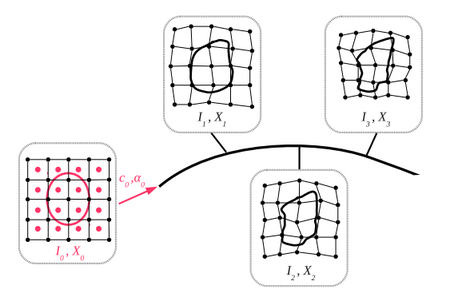
The geodesic regression model leverages image and shape data together to estimate a single time-dependent deformation of the ambient space. By analogy with linear regression, we estimate a baseline shape configuration (intercept) and deformation parameters (slope) in order to minimize the distance between the model and the observed shapes.

The deformations in our model are diffeomorphisms (smooth, one-to-one, and invertible transformation of space) which act on shapes embedded in the ambient 2D or 3D space. The group of diffeomorphisms forms an infinite dimensional manifold. This is the space in which our model is geodesic, a minimal energy curve on the manifold where each point along the curve is a diffeomorphism.

We call this continuous curve of diffeomorphisms a geodesic flow of diffeomorphisms, which is conveniently parameterized through a tangent space representation. The geodesic is fully described by a vector field in Euclidean space (the tangent space at a point on the manifold), called the initial momenta. From initial momenta, we can travel along the geodesic and construct diffeomorphisms by solving a system of coupled ODEs. The flow of diffeomorphisms act continuously on the embedded shapes, starting with the baseline shape configuration, resulting in continuous shape trajectories.

Therefore, the model is fully parameterized by an initial baseline shape configuration (intercept) and initial momenta (slope). Model estimation consists of estimating a baseline shape configuration, initial momenta as well as their spatial locations, called control points. The control point formulation allows momenta to be located in areas which undergo the most dynamic changes, rather than being restricted by any particular shape representation, located at the voxels of the image for instance. A graphical overview of geodesic regression is shown in Fig. 1.

Fig. 1. Conceptual overview of geodesic regression on multi-object complexes containing both image and shape data. The framework estimates parameters at t = 0 which consist of the baseline image I0 and shape X0 along with the deformation model parameterized by control points c0 and initial momenta α0 such that overall distance between the deformed objects and the observations are minimal.

For details on the mathematical formulation and estimation of model parameters given observed data, see [1,2,3].

Experimental Results for Shapes

Pediatric Subcortical Development

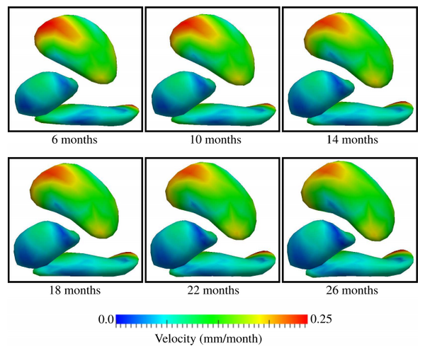
We investigate the application of geodesic shape regression to model pediatric subcortical development. Three subcortical shapes are considered as a multi-object shape complex: putamen, amygdala, and hippocampus. The structures were obtained from MRI of a healthy child scanned at approximately 9, 13, and 24 months of age. Regression was conducted on all shapes simultaneously, resulting in one deformation of the ambient space.

Several snapshots of the evolution of subcortical structures is shown in Fig. 2, with estimated baseline shape shown at 6 months. From 6 to 26 months, all subcortical structures increase in size, with the putamen demonstrating the most dramatic growth. The evolution of the putamen is characterized by accelerated growth at the superior anterior and inferior posterior regions, while the hippocampus grows mostly at the extreme posterior region, expanding and bending at the tip. The geodesic model is able to capture interesting non-linear growth patterns with few parameters; the full time evolution is modeled by three baseline shapes and 126 momenta vectors.

Fig. 2. Snapshots of subcortical shape evolution after geodesic regression on a multi-object complex: putamen, amygdala, and hippocampus.

This experiment demonstrates the applicability of the geodesic model in characterizing pediatric subcortical development. Our regression framework simultaneously handles multiple shapes, including those with complex geometry. Multi-object regression allows for a more complete analysis, compared to an independent treatment of each subcortical structure, which ignores potentially important spatial relationships between structures.

White Matter Fibers in Early Brain Development

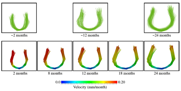
we study early brain development by considering the evolution of white matter connections from birth to 2 years of age. For this experiment, we have diffusion tensor imaging (DTI) data from 17 subjects with scans obtained at clustered time points of 2 ± 2, 12 ± 2 months, and 24 ± 2 months. We extract the genu fiber tract from each DTI. In our experiment, we use 26 genu fiber tracts which are represented as a collection of 3D curves. By considering fiber geometry obtained from multiple subjects, the estimated geodesic model can be considered as the development of the genu tract for an average child.

The average development of the genu tract estimated by our geodesic model is summarized in Fig. 3, which shows several snapshots on the genu fibers over time. The elongation of the fibers reflects the myelination process that occur during early development, where myelin sheaths grows to cover white matter regions outward to the cortex. Our geodesic regression framework handles the multiple fiber structure that form the genu fiber bundle.

Fig. 3. Average development of genu fiber tract from 2 to 24 months. Top row shows observed data for all subjects, which is clustered around 2, 12, and 24 months. Bottom row shows genu fiber tracts estimated from geodesic regression at several time points with velocity of fiber development displayed on the surface of the estimated fibers.

Experimental Results for Images and Shapes

Pediatric Brain Development

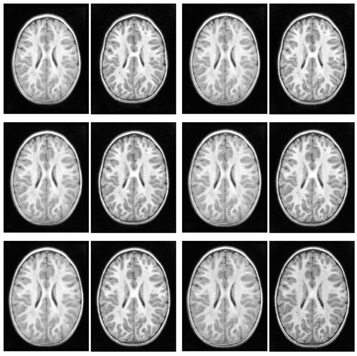
We explore the impact of joint image and shape regression in modeling pediatric brain development. The data consists of T1W images of the same healthy child observed at 6, 12, and 25 months of age. Regression on images alone is difficult in this case due to the very low contrast in the 6 month old image. Despite the low contrast, tissue segmentations can still be reliably and consistently estimated [10]. We estimate a geodesic model using only T1W images and a model jointly on images and white matter surfaces to emphasize the development of the tissue interface.

The results of geodesic regression are shown for several snapshots in time in Fig. 4. The model estimated using only images mostly captures the scale change, but does not capture much deformation in the interior of the brain. The model estimated jointly on image and shape captures more detailed development as white matter stretches and expands.

Fig. 4. Images and deformations estimated by geodesic regression using images alone (top) and jointly on images and white matter surfaces (bottom). Regression jointly on image and shape results in a more realistic evolution which captures detailed changes in brain tissue in addition to the increase in brain size. In both cases, geodesic regression was estimated backwards in time.

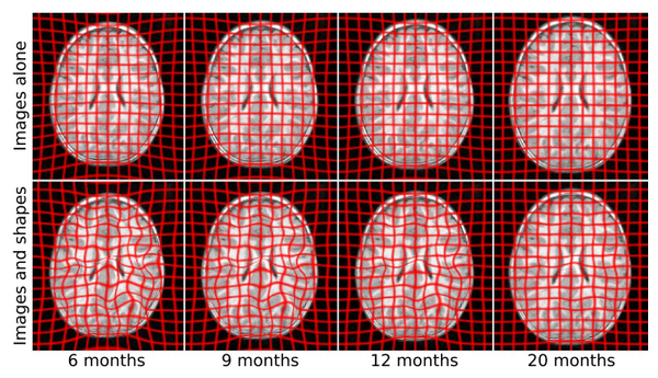
The differences between the two models is most evident when viewed as a movie, shown in Fig. 5.

Fig. 5. Animation of the models estimated with images only (left) and with images and white matter surfaces (right).

Neurodegeneration in Huntington’s Disease

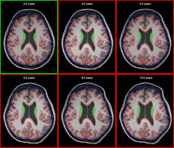
We investigate the application of joint image and shape regression to Huntington’s disease (HD) where accurate 4D models are needed to measure the effectiveness of therapies or drug treatments. In HD, degeneration of the caudate has been shown to be significant. Here we explore T1W image data from a single patient diagnosed with HD scanned at 58, 59, and 60 years of age. Sub-cortical structures are segmented, manually verified, and cleaned. Models are estimated using only T1W images as well as T1W images plus caudate surfaces.

The trajectory of caudate volume extracted after regression is shown in Fig. 6. The model estimated from images alone fails to capture the volume loss observed in both caudates, and rather, shows an increase in right caudate volume. By incorporating caudate shape data in model estimation, we are able to capture the shrinking of the caudates. The corresponding expansion of the ventricles is also captured, shown in Fig 4, due to the inclusion of imaging data. By incorporating shape and image information jointly, we are able to model both the expansion of the ventricles and the degeneration of the caudates. Accurate models of change are essential when extrapolating beyond the observation time interval, which can provide insight into disease progression.

Fig. 6. Top) Evolution estimated on images alone. Evolution of caudates are not estimated, but instead we shoot the baseline caudate shapes along the estimated geodesic. Bottom) Evolution estimated jointly using images and caudate shapes. Regression on images alone results in a slight expansion of ventricles, but does not capture the shrinking of caudates. By incorporating imaging and shape data, we capture both the expansion of ventricles and the shrinking of caudates.

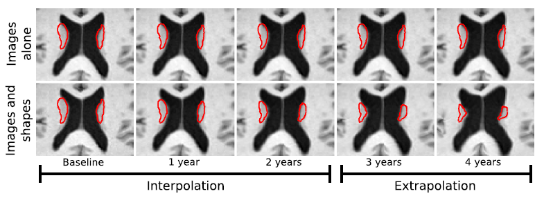
Fig. 7 shows an animation of model estimated for a single subject with Huntington's disease, showing interpolation inside the window of observed data as well as extrapolation 10 years from the baseline observation.

Fig. 7. Animation of a model estimated with image and shape data. A green border around the image represents interpolation within the observation interval (3 years). A red border represents extrapolation out to 10 years from baseline.

Sparse Parameterization of Diffeomorphisms

The control point formulation provides a sparse representation of diffeomorphisms, separating the model parameters from the shape representations. Optimal control point locations are estimated, and the number of control points is chosen by the user. This is in contrast to model parameters tied to a specific shape representation, located at every shape vertex or every image voxel, for example. The number of model parameters should reflect the complexity of anatomical changes in time rather than the sampling of the images.

However, even with the control point formulation, the dynamics of image evolution are likely characterized by considerably fewer parameters than the number of initial control points. We introduce a sparsity prior into model estimation. An upper bound on the dimensionality of the deformation is chosen by the user, and a L1 penalty selects the most relevant subset of initialmomenta, those that describe the most salient changes over time.

Synthetic Evolution

We explore a synthetic image time series. The synthetic data, shown in Fig. 8, was generated by shooting the baseline image along predefined initial momenta. The resulting evolution is therefore geodesic, which serves as a best case scenario for our model. We explore the impact of the sparsity parameter by estimating several geodesic models with a range of values for sparsity.

Fig. 8. Synthetic image evolution generated by shooting the baseline image (far left) along predefined initial momenta, constraining the resulting evolution to be geodesic.

The estimated baseline shape and initial momenta for increasing values of sparsity parameter are shown in Fig. 9. Increasing the sparsity parameter results in a decrease in the number of control points, leading to a more compact representation of the dynamics of shape change over time. The momenta which remain for high values of the sparsity parameter represent the areas that undergo the most dynamic changes. In that sense, these momenta hold the most important information about the trajectory of image evolution.

Fig. 9. Baseline shape and initial momenta estimated for several values of sparsity parameter.. An increase in the sparsity parameter leads to a more compact representation, with momenta located in areas of dynamic change over time.

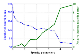
Fig. 3 shows the impact the sparsity parameter has on the number of control points as well as the accuracy in which the estimated evolution matches observed data. We can obtain a 43% decrease in the number of control points for less than a 2% relative increase in data matching error, or a 70% decrease in control points for a 10% cost. We obtain a reasonable model of shape change with as few as 67 momenta, compared to 79804 momenta (one for every pixel) for dense deformation models.

Fig. 10. Impact of the sparsity parameter for the synthetic experiment . There is a range of values of the sparsity parameter which result in a considerable decrease in the number of control points for only minimal increase in the relative error of the data matching term.

Literature

[1] Fishbaugh, J., Prastawa, M., Gerig, G., Durrleman, S. Geodesic regression of image and shape data for improved modeling of 4D trajectories. IEEE International Symposium on Biomedical Imaging (ISBI '14)

[2] Fishbaugh, J., Prastawa, M., Gerig, G., Durrleman, S. Geodesic image regression with a sparse parameterization of diffeomorphisms. Geometric Science of Information (GSI '13). LNCS vol 8085, pp. 95-102. (2013)

[3] Fishbaugh, J., Prastawa, M., Gerig, G., Durrleman, S. Geodesic shape regression in the framework of currents. Proc. of Information Processing in Medical Imaging (IPMI '13). Vol 23, pp. 718-729. (2013)

Key Investigators

• Utah: James Fishbaugh, Marcel Prastawa, Guido Gerig
• INRIA/ICM, Pitie Salpetriere Hospital: Stanley Durrleman

Back to Utah 2 Algorithm Core